#How and Why CNNs work
#Recap How Neural Network make Classifications and Update weights

How and Why CNNs work

To really grasp Convolutional Neural Networks (CNNs), you have to step away from the math for a second and look at the physical intuition. The architecture of a CNN is actually heavily inspired by how the human visual cortex works.

Let’s use a practical example: Training a CNN to recognize a Car.

When you look at a car, you don't process every single microscopic photon of color at once. Your brain subconsciously looks for edges, combining those edges into shapes (circles for wheels, squares for windows), and combining those shapes into a final concept (a car). A CNN does exactly the same thing layer by layer.

This is the intuition behind each step of the process.

1. The Convolutional Layer (CONV): The Detective

The Purpose: Feature extraction. This layer scans the image to find specific visual patterns.

The Intuition:

Imagine you are a detective looking at a massive crime scene photo, but you are only allowed to look through a tiny 3x3 inch magnifying glass. You slide this magnifying glass across the entire image, left to right, top to bottom.

In a CNN, that magnifying glass is the filter (or kernel).

• Early CONV layers have simple filters that look for basic things: a vertical edge, a horizontal line, or a splash of red.

• As the network gets deeper, it stacks these layers. Deeper CONV layers combine those basic lines to look for complex concepts. A filter in layer 3 might specifically light up when it slides over a "wheel" or a "windshield."

Every time the filter finds what it is looking for, it creates a "hotspot" on an activation map. So, an activation map is just a filtered version of the image that highlights where a specific feature exists.

2. The ReLU Activation Layer: The Light Switch

The Purpose: To introduce non-linearity by removing negative values.

The Intuition:

After the Convolution layer slides its filter over the image, it calculates a score. A high positive score means, "Yes, I definitely found a wheel here!" A negative score means, "No, this looks like the exact opposite of a wheel."

ReLU (Rectified Linear Unit) acts as a harsh bouncer. Its rule is simple: Keep positive numbers exactly as they are, but turn all negative numbers to zero.

Why? Because in the context of visual features, a negative feature doesn't make sense. You either found the wheel, or you didn't. By turning negatives to zero, ReLU acts like a light switch, turning the signal "ON" where a feature exists and "OFF" where it is just background noise. This prevents the network from just being a giant, rigid linear math equation.

3. The Pooling Layer (POOL): The Summarizer

The Purpose: Downsampling, reducing computation, and adding spatial invariance.

The Intuition:

Imagine you are looking at a highly detailed photograph, and then you step back and squint your eyes. You lose the exact, crisp details, but you can still easily tell that there is a car in the photo.

Pooling (specifically Max Pooling) is the mathematical equivalent of squinting. It takes a small block of pixels (e.g., a 2x2 grid) from the activation map, throws away the smaller numbers, and only keeps the maximum value (the strongest signal).

This does two massive things for the network:

1. Saves Memory: It shrinks the size of the image data by 75% at every step, making the model fast enough to actually run.

2. Creates "Translation Invariance": You don't want your model to break just because the car in the photo is shifted two pixels to the left. Because Max Pooling summarizes a region, it tells the network: "I don't care about the exact microscopic coordinate of the wheel, I just care that a wheel exists somewhere in this general bottom-left area."

4. The Fully Connected Layer (FC): The Jury

The Purpose: To take all the extracted, high-level features and make the final classification.

The Intuition:

At the very end of the network, the 3D maps of features (the outputs of the CONV and POOL layers) are flattened into a single, long 1D list of numbers.

This list is handed over to the Fully Connected layer, which acts like a jury in a courtroom. The FC layer looks at the evidence gathered by the previous layers:

• Evidence 1: Strong signal for wheels.

• Evidence 2: Strong signal for a windshield.

• Evidence 3: Strong signal for a license plate.

The neurons in the Fully Connected layer are trained to weigh this specific combination of evidence and cast their vote. Based on the weights, the jury decides: "Given these features, we classify this image as a Car with 94% probability."

Recap: How Neural Network make Classifications and Update weights

This is a quick, high-yield revision of how a Neural Network actually learns.

The simplest analogy: Forward propagation is the student taking the exam and making a guess. Backward propagation is the teacher grading the exam, showing the student where they went wrong, and the student adjusting their knowledge for the next test.

1. Forward Propagation (The Prediction Phase)

In forward propagation, information flows strictly from left to right (from the input layer, through the hidden layers, to the output layer). The network is essentially making its best mathematical guess based on its current weights.

The Process (for a specific layer $l$):

1. Linear Transformation: The layer takes the activations ($A$) from the previous layer, multiplies them by its own weight matrix ($W$), and adds a bias ($b$).

   $$Z^{[l]}=W^{[l]}{A}^{[l-1]}+b^{[l]}$$

2. Non-Linear Activation: The raw output ($Z$) is passed through an activation function $g$ (like ReLU, Sigmoid, or Tanh) to introduce non-linearity, producing the activation for the current layer.

   $$A^{[l]}=g(Z^{[l]})$$

   (Note: For the very first hidden layer, the input $A^{[l-1]}$ is just your raw data $X$.)

3. The Loss Calculation: Once the signal reaches the final output layer, it produces a prediction ($\hat{y}$ or $A^{[L]}$). The network then compares this prediction to the true label ($Y$) using a Loss Function (like Mean Squared Error or Cross-Entropy) to calculate the total error.

Crucial detail: During forward propagation, the network must cache (save) the $Z$ and $A$ values at every single layer. It will need these specific numbers later to calculate the gradients during backprop.

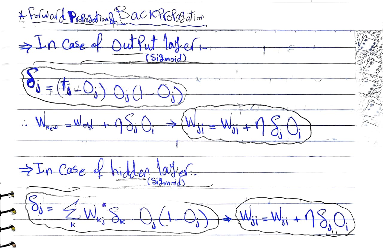
2. Backward Propagation (The Learning Phase)

This is where the actual "learning" happens. Information flows from right to left (from the output layer back to the input layer). The goal is to figure out exactly how much each specific weight and bias contributed to the final error, so we know how to fix them.

The Core Engine: The Chain Rule of Calculus

Because a neural network is just a massive composite math function ($f(g(h(x)))$), backprop uses the chain rule to calculate the partial derivatives (gradients) of the Loss function with respect to every single weight ($W$) and bias ($b$).

The Process (moving backwards from layer $l$ to $l-1$):

1. Calculate the Error at the Current Layer ($dZ$): How much was the raw output $Z$ responsible for the error? This relies on the derivative of the activation function $g^{\prime }$.

   $$d{Z}^{[l]}=d{A}^{[l]}\ast g^{\prime }(Z^{[l]})$$

2. Calculate the Gradients for Weights and Biases: Now that we know the error at this layer, we determine how much to change $W$ and $b$. (Here, $m$ is the number of examples in the batch).

   $$d{W}^{[l]}=\frac{1}{m}d{Z}^{[l]}{A}^{[l-1]T}$$$$d{b}^{[l]}=\frac{1}{m}\sum d{Z}^{[l]}$$

3. Pass the Error Backwards ($dA$): We calculate the error that needs to be passed back to the previous layer so the cycle can continue.

   $$d{A}^{[l-1]}=W^{[l]T}d{Z}^{[l]}$$

By: Ibrahim Reda

3. The Weight Update (The Optimization)

Once backpropagation reaches the very first layer, the network has successfully computed the gradients ($dW$ and $db$) for every single parameter in the entire model.

Now, the network hands these gradients over to an Optimizer (like standard Gradient Descent, RMSProp, or Adam—which we covered in Module 4). The optimizer updates the weights to minimize the loss for the next epoch.

Using standard Gradient Descent with a learning rate of $\alpha$:

After this update, the network grabs the next batch of data, and the entire Forward $\to$ Loss $\to$ Backward $\to$ Update cycle repeats until the model converges!