Lecture 2 Examples

Lecture 2 Examples#1. Categorical Naïve Bayes (Play Tennis Dataset)
#2. Gaussian Naïve Bayes (Numerical Data)
#3. Principal Component Analysis (PCA)
#More On Naive Bayes

1. Categorical Naïve Bayes (Play Tennis Dataset)

The Scenario:

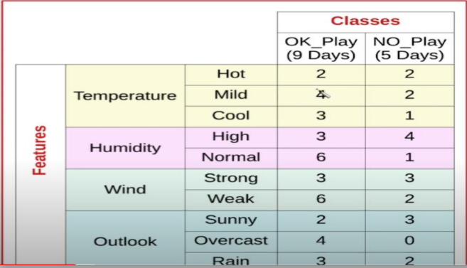
We have historical data on whether a tennis game was played (OK_Play = 9 days, NO_Play = 5 days, Total = 14 days).

Pasted image 20260330221457.png

We need to classify a new, unseen day ( $Z$ ) with the following conditions:

Outlook: Sunny
Temperature: Cool
Humidity: High
Wind: Strong

Step 1: Calculate the Probabilities for OK_Play

We multiply the likelihood of each feature occurring when the game was played by the prior probability of playing at all.

$P (S u n n y | O K_P l a y) = 2 / 9$
$P (C o o l | O K_P l a y) = 3 / 9$
$P (H i g h | O K_P l a y) = 3 / 9$
$P (S t r o n g | O K_P l a y) = 3 / 9$
Prior: $P (O K_P l a y) = 9 / 14$

Pasted image 20260330221512.png

Equation:

P (O K_P l a y | Z) \propto (\frac{2}{9} \times \frac{3}{9} \times \frac{3}{9} \times \frac{3}{9}) \times \frac{9}{14} = 0.0053

Step 2: Calculate the Probabilities for NO_Play

We do the same for when the game was not played.

$P (S u n n y | N O_P l a y) = 3 / 5$
$P (C o o l | N O_P l a y) = 1 / 5$
$P (H i g h | N O_P l a y) = 4 / 5$
$P (S t r o n g | N O_P l a y) = 3 / 5$
Prior: $P (N O_P l a y) = 5 / 14$

Equation:

P (N O_P l a y | Z) \propto (\frac{3}{5} \times \frac{1}{5} \times \frac{4}{5} \times \frac{3}{5}) \times \frac{5}{14} = 0.0206

Result: Since 0.0206 is greater than 0.0053, the model classifies this new day as NO_Play.

2. Gaussian Naïve Bayes (Numerical Data)

The Scenario:

Pasted image 20260330222240.png

Recall: the marginalization rule "total probability", is when you calculate the probability of some variable, by summing over the joint distribution of all possible values of another variable

P (a_{i}) = \sum_{j = 1}^{N_{b-classes}} P (a_{i}, b_{j})

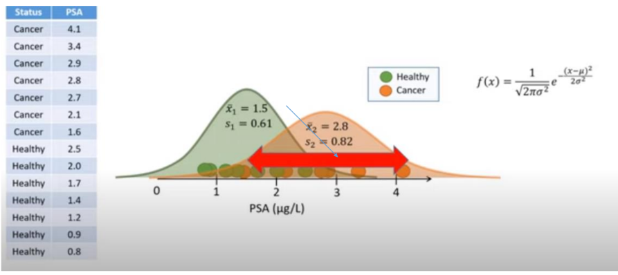
Instead of counts, we are dealing with continuous numbers (PSA level and Age) to classify a patient as Healthy or Cancer. Because we assume the features follow a normal distribution, we plug our values into the Gaussian Probability Density Function:

f (x) = \frac{1}{\sqrt{2 π σ^{2}}} e^{- \frac{(x - μ)^{2}}{2 σ^{2}}}

Test Patient: PSA = 2.6, Age = 70
Priors: $P (H e a l t h y) = 0.5$ , $P (C a n c e r) = 0.5$

Step 1: Calculate Likelihoods for Healthy

Using the mean ( $μ$ ) and standard deviation ( $σ$ ) from the Healthy training data:

PSA Likelihood: $μ = 1.5, σ = 0.61 \to P (P S A = 2.6 | H e a l t h y) = 0.13$
Age Likelihood: $μ = 66, σ = 4.58 \to P (A g e = 70 | H e a l t h y) = 0.059$

Posterior Numerator (Healthy):

P (H e a l t h y) \times P (P S A | H e a l t h y) \times P (A g e | H e a l t h y)

0.5 \times 0.13 \times 0.059 = 0.004

Step 2: Calculate Likelihoods for Cancer

Using the mean and standard deviation from the Cancer training data:

PSA Likelihood: $μ = 2.8, σ = 0.82 \to P (P S A = 2.6 | C a n c e r) = 0.47$
Age Likelihood: $μ = 67, σ = 6.45 \to P (A g e = 70 | C a n c e r) = 0.055$

Posterior Numerator (Cancer):

P (C a n c e r) \times P (P S A | C a n c e r) \times P (A g e | C a n c e r)

0.5 \times 0.47 \times 0.055 = 0.013

Result: Since 0.013 is greater than 0.004, the model classifies the patient as having Cancer.

3. Principal Component Analysis (PCA)

The Scenario:

We want to reduce the dimensionality of a 2D dataset while preserving the most important variance.

Data Points: (2, 1), (3, 5), (4, 3), (5, 6), (6, 7), (7, 8)

Step 1: Calculate the Mean Vector ( $μ$ )

Find the average of all $X$ values and all $Y$ values.

μ = [\begin{matrix} (2 + 3 + 4 + 5 + 6 + 7) / 6 \\ (1 + 5 + 3 + 6 + 7 + 8) / 6 \end{matrix}] = [\begin{matrix} 4.5 \\ 5 \end{matrix}]

Step 2: Subtract the Mean

Center the data around the origin by subtracting the mean from every point.

$P_{1} : (2 - 4.5, 1 - 5) = (- 2.5, - 4)$
...repeat for all points...
$P_{6} : (7 - 4.5, 8 - 5) = (2.5, 3)$

Step 3: Calculate the Covariance Matrix

Compute $(x_{i} - μ) (x_{i} - μ)^{T}$ for each point, sum them up, and divide by the number of points ( $n = 6$ ) to find how the variables vary together.

C o v a r i a n c e M a t r i x = [\begin{matrix} 2.92 & 3.67 \\ 3.67 & 5.67 \end{matrix}]

Step 4: Find Eigenvalues and Eigenvectors

Solve the characteristic equation $| M - λ I | = 0$ (where $M$ is the covariance matrix) to find the eigenvalues ( $λ$ ).

λ^{2} - 8.59 λ + 3.09 = 0

Eigenvalues: $λ_{1} = 8.22$ (Principal), $λ_{2} = 0.38$ (We drop this small one to reduce dimensions).

Next, we solve $M X = λ X$ using the dominant eigenvalue ( $λ_{1} = 8.22$ ) to get the principal Eigenvector.

P r i n c i p a l C o m p o n e n t = [\begin{matrix} 2.55 \\ 3.67 \end{matrix}]

Step 5: Project the Data

Finally, we recast the original data points onto this new 1D principal component line by taking the dot product.

Projecting Point 1 (2, 1): $(2 \times 2.55) + (1 \times 3.67) = 8.77$
Projecting Point 2 (3, 5): $(3 \times 2.55) + (5 \times 3.67) = 26.00$
(This creates your new, 1-dimensional reduced dataset!)

More On Naive Bayes

Why Naive Bayes

Its main strength is requiring less training data, while its primary weakness is the "naive" assumption that all features are independent, which rarely holds true in real-world scenarios.

Pros of Naive Bayes:

Fast and Scalable: Highly efficient in training and prediction, suitable for real-time applications and large datasets.
Performance with Less Data: Performs well with small training sets and high-dimensional data (e.g., text categorization).
Simplicity: Easy to implement and understand.
Handles Multi-class: Effective for multi-class prediction tasks.
Robust to Irrelevant Features: Not sensitive to irrelevant features in the dataset.

Cons of Naive Bayes:

Independence Assumption: Assumes features are independent, which rarely holds true. If features are correlated, performance can degrade.
Zero-Frequency Problem: If a categorical variable has a category in the test set that was not observed in the training set, the model will assign a zero probability.
Not Ideal for Complex Relationships: Struggles to capture complex relationships or dependencies between features.
Data Scarcity: Requires sufficient data for each class to accurately estimate probabilities.

Common Use Cases:

Spam filtering
Sentiment analysis
Document/Article classification
Real-time prediction systems

A \equiv y = C_{i}

B \equiv x = x_{i}

P (y = C_{i} | x = x_{j}) = \frac{P (x = x_{j} | y = C_{i}) P (y = C_{i})}{P (x = x_{j})}

{\hat{y}}_{j} = C_{{argmax}_{i} P (y = C_{i} | x = x_{j})}

P (y = C_{i} | x_{1 j}, x_{2 j}, x_{3 j}, \dots, x_{d j}) = \frac{P (x_{1 j}, x_{2 j}, x_{3 j}, \dots, x_{d j} | y = C_{i}) P (y = C_{i})}{P (x_{1 j}, x_{2 j}, x_{3 j}, \dots, x_{d j})}

Naive Assumption: We assume that all features are mutually exclusive / uncorrelated
Recall: the marginalization rule "total probability", is when you calculate the probability of some variable, by summing over the joint distribution of all possible values of another variable

P (a_{i}) = \sum_{j = 1}^{N_{b-classes}} P (a_{i}, b_{j})

P (A | B) = P (A)

Therefore:

P (y = C_{i} | x_{1 j}, x_{2 j}, x_{3 j}, \dots, x_{d j}) = \frac{P (x_{1 j} | y = C_{i}) P (x_{2 j} | y = C_{i}) P (x_{3 j} | y = C_{i}) \dots P (x_{d j} | y = C_{i}) P (y = C_{i})}{P (x_{1 j}) P (x_{2 j}) P (x_{3 j}) \dots P (x_{d j})}

The "Naivety"

Calculating the exact joint probability of many interacting variables " for calculating $P (B)$ , and $P (B | A)$ " requires exponential computational complexity ( $O (2^{n})$ ). The Naïve Bayes classifier drastically simplifies this by making a strong assumption: all features are conditionally independent of each other, given the class label.

Mathematically, it changes the complex joint probability into a simple product of individual probabilities: $P (y | x_{1}, \dots, x_{n}) \propto P (y) \prod_{i = 1}^{n} P (x_{i} | y)$
While this assumption is "naïve" because real-world variables are almost always correlated, the algorithm is famously robust. It often achieves high accuracy in classification tasks (like spam filtering) with exceptionally low computational overhead.

When making a decision between two classes ( $w_{1}$ and $w_{2}$ ) given an observation $x$ , the rule is to choose $w_{1}$ if $P (w_{1} | x) > P (w_{2} | x)$ .

Normalization

The Marginalization Rule (often called the Law of Total Probability) is the mathematical engine behind the denominator in Bayes' Theorem. In the context of machine learning, it is what allows us to convert raw, abstract scores into clean, readable percentages that sum up to 100% (or 1.0).

Bayes theorem with marginal probability, AI generated

Here is Bayes' formula:

P (C l a s s | F e a t u r e s) = \frac{P (F e a t u r e s | C l a s s) \times P (C l a s s)}{P (F e a t u r e s)}

The denominator, $P (F e a t u r e s)$ , is the marginal probability. It represents the total probability of seeing this specific exact combination of features across all possible classes in your dataset.

How to Calculate the Marginal Probability with Multiple Features

When you have multiple features (like Temperature, Humidity, Wind, or Age, PSA), calculating the exact probability of that specific combination occurring in the wild is extremely difficult.

Instead, the Marginalization Rule lets us calculate it by summing up the "numerators" of all our possible classes.

The formula for the marginal probability becomes:

P (F e a t u r e s) = \sum_{k = 1}^{n} P (F e a t u r e s | C l a s s_{k}) \times P (C l a s s_{k})

The Normalization Trick (Step-by-Step)

Because the marginal probability (the denominator) is the exact same for every class you are evaluating, you do not actually need to compute it right away. You can just calculate the numerators, sum them up, and use that sum to normalize your results.

Let's use the numerical Healthy vs. Cancer example from the lecture slides to see this in action!

1. Calculate the Numerator for Class A (Healthy)

We multiply the Prior by the Likelihoods of the features (PSA = 2.6):

Numerator (Healthy) = $P (H e a l t h y) \times P (P S A = 2.6 | H e a l t h y)$
Numerator (Healthy) = $0.5 \times 0.13 = 0.065$

2. Calculate the Numerator for Class B (Cancer)

Numerator (Cancer) = $P (C a n c e r) \times P (P S A = 2.6 | C a n c e r)$
Numerator (Cancer) = $0.5 \times 0.47 = 0.235$

3. Apply the Marginalization Rule (Find the Denominator)

To find the total marginal probability of someone having a PSA of 2.6, we simply add the numerators together:

Marginal Probability = $0.065 + 0.235 = 0.300$

4. Normalize to get the Final Probabilities

Now, divide each class's numerator by the marginal probability to get the true, normalized posterior probabilities:

Final Probability (Healthy): $0.065 / 0.300 = 0.21$ (or 21%)
Final Probability (Cancer): $0.235 / 0.300 = 0.783$ (rounded to 79% in the slides)

By dividing by the marginalized sum, you force the probabilities to scale proportionally so that $0.21 + 0.79 = 1.0$ . This tells your model not just which class is more likely, but exactly how confident it should be in that prediction!

To use that exact marginalization rule for multiple features, we have to rely on the "Naïve" part of the Naïve Bayes algorithm: Conditional Independence.

If you have a dataset with multiple features (like PSA and Age, or Outlook, Temperature, Humidity, and Wind), trying to find the true, real-world probability of that exact combination happening all at once— $P (F e a t u r e s)$ —is nearly impossible. You would need a massive dataset to find enough people who are exactly 70 years old and have a PSA of exactly 2.6 just to count them.

To get around this, Naïve Bayes assumes that every feature is completely independent of the others, as long as you already know the class.

Here is how that theoretical breakdown works mathematically.

1. Breaking Down the Likelihood

Because we assume the features are independent, the joint probability of all features given a specific class— $P (F e a t u r e s | C l a s s_{k})$ —simply becomes the product of their individual probabilities:

P (F e a t u r e s | C l a s s_{k}) = P (F e a t u r e_{1} | C l a s s_{k}) \times P (F e a t u r e_{2} | C l a s s_{k}) \times \dots \times P (F e a t u r e_{m} | C l a s s_{k})

2. Expanding the Marginalization Rule

Now, we take that expanded, multiplied likelihood and plug it back into the formula you provided. To find the total marginal probability of seeing this specific combination of features across your entire dataset, you calculate this product for every single class and add them all together:

P (F e a t u r e s) = \sum_{k = 1}^{n} ([P (F e a t u r e_{1} | C l a s s_{k}) \times \dots \times P (F e a t u r e_{m} | C l a s s_{k})] \times P (C l a s s_{k}))

3. A Theoretical Example

Let's apply this directly to the two-feature numerical example from your lecture (PSA = 2.6 and Age = 70) to see the full equation in action.

We have two classes ( $n = 2$ ): Healthy and Cancer.

Part A: Calculate the inner term for Class 1 (Healthy)

{Term}_{1} = P (P S A = 2.6 | H e a l t h y) \times P (A g e = 70 | H e a l t h y) \times P (H e a l t h y)

Part B: Calculate the inner term for Class 2 (Cancer)

{Term}_{2} = P (P S A = 2.6 | C a n c e r) \times P (A g e = 70 | C a n c e r) \times P (C a n c e r)

Part C: Sum them up for the Marginal Probability

P (P S A = 2.6 and A g e = 70) = {Term}_{1} + {Term}_{2}

Once you have that final summed number, you have successfully calculated your denominator! You then divide ${Term}_{1}$ by this denominator to get the final normalized percentage for Healthy, and divide ${Term}_{2}$ by this denominator to get the final normalized percentage for Cancer.

بالبلدي لو عايز زتونة الحل, لو طلب منك تعمل normalization, اجمع البسط بتاع كل الاحتمالات اللي حسبتها "ال likelihoods في ال priors بتاعت كل كلاس, سواء بقي كانت one or more than one feature"