Lecture 4 - Optimizers, Hyperparameter Tuning

1. Performance Evaluation

Before you can improve a model, you need to know how to measure its current performance. The lecture highlights that as model complexity increases, training error naturally decreases, but test error will eventually start to increase—creating a convex curve that represents overfitting.

Evaluating Regression Models

For regression (predicting continuous values), the slides define two primary metrics:

Mean Absolute Error (MAE): The average of the absolute differences between predictions and actual values. Closer to 0 is better.
$M A E = \frac{1}{m} \sum_{i = 1}^{m} | y_{i} - {\hat{y}}_{i} |$
Mean Squared Error (MSE): The average of the squared differences. (Note: The slide formula uses ${\overset{―}{y}}_{i}$ , which typically denotes the mean, but in this context, it represents the predicted value comparable to ${\hat{y}}_{i}$ ).
$M S E = \frac{1}{m} \sum_{i = 1}^{m} (y_{i} - {\overset{―}{y}}_{i})^{2}$

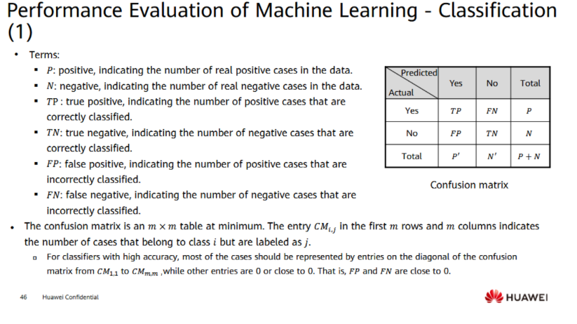
Evaluating Classification Models

For classification, performance is broken down using a Confusion Matrix, which tracks:

True Positives (TP) / True Negatives (TN): Cases your model classified correctly.
False Positives (FP) / False Negatives (FN): Cases your model classified incorrectly.

From this matrix, we derive several critical formulas:

Accuracy: $\frac{T P + T N}{P + N}$ (Overall correctness).
Error Rate: $\frac{F P + F N}{P + N}$ (Overall incorrectness).
Recall (Sensitivity): $\frac{T P}{P}$ (Out of all actual positives, how many did we find?) "Completeness" .
Precision: $\frac{T P}{T P + F P}$ (Out of all predicted positives, how many were actually positive?) "Soundness" .
F1 Score: $\frac{2 \times p r e c i s i o n \times r e c a l l}{p r e c i s i o n + r e c a l l}$ (The harmonic mean of precision and recall, useful when classes are imbalanced).

Pasted image 20260331014652.png

2. Hyperparameter Tuning

As discussed in previous lectures, hyperparameters are external configurations set manually by the user (like the learning rate $η$ , $K$ in KNN, or the number of trees in a Random Forest).

The standard search process is:

Divide data into train, validation, and test sets.
Optimize internal parameters on the training set.
Search for the best hyperparameters using the validation set.
Alternate until finalized, then do a final assessment on the test set.

Search Methods:

Grid Search: Tests every single possible combination on a manually specified grid. It is highly exhaustive but extremely expensive and time-consuming, making it unfeasible for deep neural networks.
Random Search: Samples random combinations from a broad range, eventually narrowing down the search area based on where the best results are found. This is much more efficient for large search spaces.

3. Optimizer Types

Optimizers are the specific algorithms used to update the weights of your model during training. They aim to accelerate convergence, prevent getting stuck in local minimums, and simplify learning rate adjustments.

1. Standard Gradient Descent Updates weights by taking a step in the negative direction of the gradient.

w_{k + 1} = w_{k} - η \nabla f_{w_{k}} (x^{i})

2. Momentum Optimizer Standard gradient descent can get stuck or oscillate. Momentum fixes this by adding a fraction of the previous update to the current update. It acts like a ball rolling down a hill, gaining inertia to push through flat spots or small bumps.

زي اي حاجة بتتدحرج علي تل, كل ما تفضل ماشي في اتجاه ثابت, تكتسب سرعة اكبر في نفس الاتجاه دهز

Δ w_{j i} (n) = - η δ_{i} x_{j} + α Δ w_{j i} (n - 1)

3. AdaGrad (Adaptive Gradient) Instead of using one global learning rate ( $η$ ) for all parameters, AdaGrad adapts the learning rate for each specific parameter. It does this by dividing the learning rate by the square root of $r_{t}$ (the accumulated sum of all past squared gradients).

r_{t} = r_{t - 1} + g_{t}^{2}

Δ w_{t} = - \frac{η}{ϵ + \sqrt{r_{t}}} g_{t}

Problem: Because $r_{t}$ strictly increases, the learning rate eventually shrinks to zero, stopping training entirely.

4. RMSProp (Root Mean Square Propagation) RMSProp fixes AdaGrad's "shrinking to zero" problem by introducing an attenuation coefficient (decay factor $β$ ). Instead of accumulating all past gradients, it keeps a moving average, allowing the model to continue learning. It is highly effective for Recurrent Neural Networks (RNNs).

r_{t} = β r_{t - 1} + (1 - β) g_{t}^{2}

5. Adam (Adaptive Moment Estimation) Adam is essentially the combination of Momentum and RMSProp, and it is the default choice for most modern deep learning.

It calculates the moving average of the gradient ( $m_{t}$ , the First Moment, like Momentum).
It calculates the moving average of the squared gradient ( $v_{t}$ , the Second Moment, like RMSProp).
It applies a bias correction ( ${\hat{m}}_{t}$ and ${\hat{v}}_{t}$ ) to prevent these values from being biased toward zero at the start of training.
The default parameters are highly stable: $β_{1} = 0.9$ , $β_{2} = 0.999$ , $ϵ = 10^{- 8}$ , and $η = 0.001$ .

تلخيصة القوانين كلها تحت اهي سيبك من القوانين اللي فوق

Here is a complete comparison of the five optimization algorithms, followed by a step-by-step numerical walkthrough for two epochs.

1. Optimizer Comparison & Equations

Each optimizer attempts to solve the core problem of standard gradient descent: finding the minimum error efficiently without getting stuck in flat regions or overshooting the target. Let $g_{t}$ represent the gradient at step $t$ , $η$ represent the learning rate, and $w_{t}$ represent the weight at step $t$ .

1. Stochastic Gradient Descent (SGD)

Concept: The baseline method. It calculates the gradient of the loss and takes a step of size $η$ in the opposite direction. It is simple but can be slow and easily gets stuck in local minima.
Equation:
$w_{t} = w_{t - 1} - η g_{t}$

2. Momentum

Concept: Adds an "inertia" term ( $v_{t}$ ). Instead of just relying on the current gradient, it remembers the direction of the previous updates (controlled by $β$ ). This helps push the optimizer through flat surfaces and dampens oscillations.
Equations:
$v_{t} = β v_{t - 1} + η g_{t}$ $w_{t} = w_{t - 1} - v_{t}$

3. AdaGrad (Adaptive Gradient)

Concept: Abandons the idea of a single global learning rate. It divides the learning rate by the square root of $G_{t}$ (the sum of all past squared gradients). Features that update frequently get smaller learning rates, while rare features get larger ones.
Equations:
$G_{t} = G_{t - 1} + g_{t}^{2}$ $w_{t} = w_{t - 1} - \frac{η}{\sqrt{G_{t}} + ϵ} g_{t}$

4. RMSProp (Root Mean Square Propagation)

Concept: Fixes AdaGrad's fatal flaw (the learning rate shrinking to zero). Instead of accumulating all past squared gradients, it uses an exponentially decaying moving average ( $s_{t}$ ), controlled by $β$ . This keeps the learning rate adaptable but prevents it from dying out.
Equations:
$s_{t} = β s_{t - 1} + (1 - β) g_{t}^{2}$ $w_{t} = w_{t - 1} - \frac{η}{\sqrt{s_{t}} + ϵ} g_{t}$

5. Adam (Adaptive Moment Estimation)

Concept: The industry standard. It combines the "inertia" of Momentum (First Moment, $m_{t}$ ) with the "adaptive learning rate" of RMSProp (Second Moment, $v_{t}$ ). It also includes bias correction ( ${\hat{m}}_{t}$ and ${\hat{v}}_{t}$ ) to ensure the initial steps aren't artificially small.
Equations:
$m_{t} = β_{1} m_{t - 1} + (1 - β_{1}) g_{t}$ $v_{t} = β_{2} v_{t - 1} + (1 - β_{2}) g_{t}^{2}$ ${\hat{m}}_{t} = \frac{m_{t}}{1 - β_{1}^{t}} and {\hat{v}}_{t} = \frac{v_{t}}{1 - β_{2}^{t}}$ $w_{t} = w_{t - 1} - \frac{η}{\sqrt{{\hat{v}}_{t}} + ϵ} {\hat{m}}_{t}$

2. Numerical Example (2 Epochs)

Let's trace these optimizers mathematically using a static gradient to see how they behave differently. For simplicity in the hand calculations, we will ignore the tiny $ϵ$ (usually 1e-8) as its only purpose is preventing division by zero.

Initial Conditions:

Starting Weight ( $w_{0}$ ): 1.0
Constant Gradient ( $g_{t}$ ): 0.5
Learning Rate ( $η$ ): 0.1
Momentum/RMSProp Factor ( $β$ ): 0.9
Adam Factors ( $β_{1}$ , $β_{2}$ ): 0.9, 0.999
All accumulators ( $v_{0}, G_{0}, s_{0}, m_{0}$ ): 0

Epoch 1 ( $t = 1$ )

SGD
- $w_{1} = 1.0 - 0.1 (0.5) = 0.95$
Momentum
- $v_{1} = 0.9 (0) + 0.1 (0.5) = 0.05$
- $w_{1} = 1.0 - 0.05 = 0.95$
AdaGrad
- $G_{1} = 0 + (0.5)^{2} = 0.25$
- $w_{1} = 1.0 - \frac{0.1}{\sqrt{0.25}} (0.5) = 1.0 - (0.2 \times 0.5) = 0.90$
RMSProp
- $s_{1} = 0.9 (0) + 0.1 (0.25) = 0.025$
- $w_{1} = 1.0 - \frac{0.1}{\sqrt{0.025}} (0.5) = 1.0 - (0.6324 \times 0.5) = 0.684$
Adam
- $m_{1} = 0.9 (0) + 0.1 (0.5) = 0.05$
- $v_{1} = 0.999 (0) + 0.001 (0.25) = 0.00025$
- ${\hat{m}}_{1} = \frac{0.05}{1 - {0.9}^{1}} = \frac{0.05}{0.1} = 0.5$
- ${\hat{v}}_{1} = \frac{0.00025}{1 - {0.999}^{1}} = \frac{0.00025}{0.001} = 0.25$
- $w_{1} = 1.0 - \frac{0.1}{\sqrt{0.25}} (0.5) = 0.90$

Epoch 2 ( $t = 2$ )

SGD
- $w_{2} = 0.95 - 0.1 (0.5) = 0.90$
Momentum
- $v_{2} = 0.9 (0.05) + 0.1 (0.5) = 0.045 + 0.05 = 0.095$
- $w_{2} = 0.95 - 0.095 = 0.855$ (Notice how the step size is increasing due to momentum)
AdaGrad
- $G_{2} = 0.25 + (0.5)^{2} = 0.50$
- $w_{2} = 0.90 - \frac{0.1}{\sqrt{0.50}} (0.5) = 0.90 - (0.1414 \times 0.5) = 0.829$ (Notice how the effective learning rate shrank)
RMSProp
- $s_{2} = 0.9 (0.025) + 0.1 (0.25) = 0.0475$
- $w_{2} = 0.684 - \frac{0.1}{\sqrt{0.0475}} (0.5) = 0.684 - (0.4588 \times 0.5) = 0.455$
Adam
- $m_{2} = 0.9 (0.05) + 0.1 (0.5) = 0.095$
- $v_{2} = 0.999 (0.00025) + 0.001 (0.25) = 0.00049975$
- ${\hat{m}}_{2} = \frac{0.095}{1 - {0.9}^{2}} = \frac{0.095}{0.19} = 0.5$
- ${\hat{v}}_{2} = \frac{0.00049975}{1 - {0.999}^{2}} = \frac{0.00049975}{0.001999} = 0.25$
- $w_{2} = 0.90 - \frac{0.1}{\sqrt{0.25}} (0.5) = 0.90 - 0.1 = 0.80$