Q1
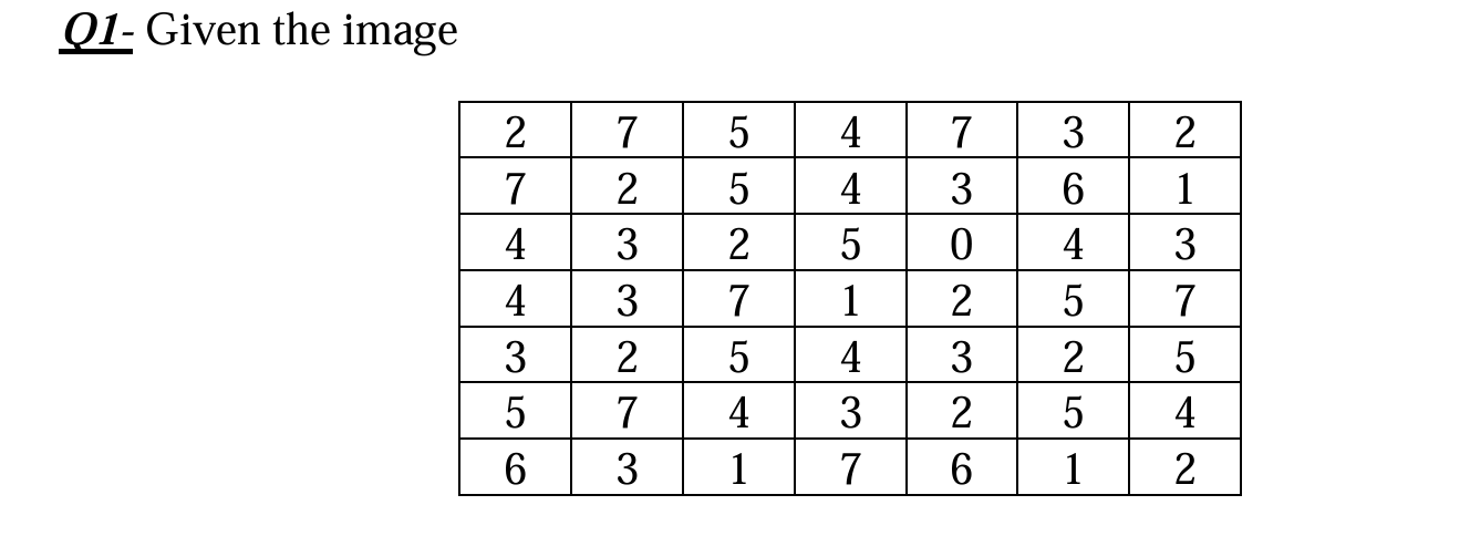
The image is a
By counting the occurrences of each pixel intensity in the given matrix, we get the base frequency data.
1.1 Histogram
The histogram
| Intensity (rk) | 0 | 1 | 2 | 3 | 4 | 5 | 6 | 7 |
|---|---|---|---|---|---|---|---|---|
| Count ( |
1 | 4 | 9 | 9 | 8 | 8 | 3 | 7 |
1.2 Cumulative Histogram
The cumulative histogram
| Intensity (rk) | 0 | 1 | 2 | 3 | 4 | 5 | 6 | 7 |
|---|---|---|---|---|---|---|---|---|
| Cumulative Count ( |
1 | 5 | 14 | 23 | 31 | 39 | 42 | 49 |
1.3 Histogram Equalization
To perform histogram equalization, we map the original intensity values
Given
Mapping Calculations:
Equalized Histogram:
Notice that original intensities 5 and 6 both map to the new intensity 6. Therefore, we add their original frequencies together (8 + 3 = 11).
| Intensity (sk) | 0 | 1 | 2 | 3 | 4 | 5 | 6 | 7 |
|---|---|---|---|---|---|---|---|---|
| New Count | 1 | 4 | 9 | 9 | 8 | 0 | 11 | 7 |
1.4 Robust Contrast Stretching (Truncation)
Truncating allows us to ignore outliers (the extreme dark and bright pixels) when setting our new minimum and maximum bounds for the contrast stretch.
Step 1: Calculate Truncation Bounds
-
10% Dark Truncation:
. Looking at the cumulative histogram, discarding the 5 darkest pixels perfectly removes all pixels with intensity 0 and 1. The new minimum valid intensity is
. -
20% Light Truncation:
. Counting from the brightest end: we have 7 pixels of intensity 7, and 3 pixels of intensity 6. Discarding the top 10 pixels removes all 7s and 6s. The new maximum valid intensity is
.
Step 2: Contrast Stretching Formula
We map the valid range
Mapping Calculations:
-
(Intensities 0, 1): Clipped to 0 since both will result in negatives -
: 0 -
: 2 -
: 5 -
: 7 -
(Intensities 6, 7): Clipped to 7
Final Stretched Histogram:
We compile the frequencies of the original pixels based on their newly mapped destinations.
-
Mapped to 0: Old intensities 0, 1, 2 (1 + 4 + 9 = 14)
-
Mapped to 2: Old intensity 3 (9)
-
Mapped to 5: Old intensity 4 (8)
-
Mapped to 7: Old intensities 5, 6, 7 (8 + 3 + 7 = 18)
| Intensity (sk) | 0 | 1 | 2 | 3 | 4 | 5 | 6 | 7 |
|---|---|---|---|---|---|---|---|---|
| New Count | 14 | 0 | 9 | 0 | 0 | 8 | 0 | 18 |
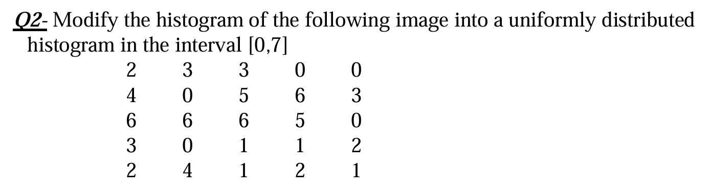
Q2
-
Total number of pixels:
-
Target interval
means our dynamic range , so . -
Our equalization multiplier will be
.
Step 1: Calculate Frequencies and Cumulative Frequencies
By counting the occurrences of each intensity (
| Intensity (rk) | 0 | 1 | 2 | 3 | 4 | 5 | 6 | 7 |
|---|---|---|---|---|---|---|---|---|
| Count ( |
5 | 4 | 4 | 4 | 2 | 2 | 4 | 0 |
| Cumulative ( |
5 | 9 | 13 | 17 | 19 | 21 | 25 | 25 |
Step 2: Apply the Equalization Formula
Now we map the original intensities (
Step 3: The Modified (Equalized) Histogram
To get the final uniformly distributed histogram, we assign the original pixel counts to their newly calculated intensity levels. Notice that both original intensities 3 and 4 are mapped to the new intensity 5, so their counts are added together (
| New Intensity (sk) | 0 | 1 | 2 | 3 | 4 | 5 | 6 | 7 |
|---|---|---|---|---|---|---|---|---|
| New Count | 0 | 5 | 0 | 4 | 4 | 6 | 2 | 4 |
Q3
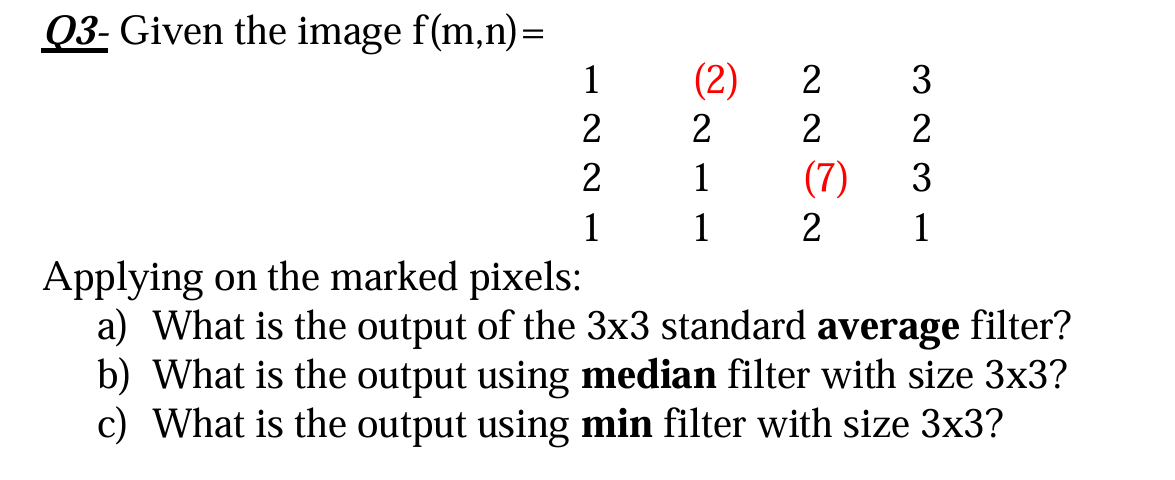
1. First Marked Pixel: (2) at position row 0, column 1
Because this pixel is on the top edge of the image, a
The
The values in this window are:
-
a) Standard Average filter: Sum the values and divide by 9.
-
-
(Note: If your class uses integer rounding, this becomes 1. If your class ignores out-of-bounds pixels entirely instead of zero-padding, the average would be
).
-
-
b) Median filter: Sort the values from lowest to highest and pick the middle (5th) value.
-
Sorted:
-
The median is 2.
-
-
c) Min filter: Select the smallest value in the neighborhood.
- The minimum is 0. (Or 1, if ignoring padded pixels).
2. Second Marked Pixel: (7) at position row 2, column 2
This is an inner pixel, so it has a complete set of 8 surrounding neighbors within the image boundaries. No padding is needed.
The
The values in this window are:
-
a) Standard Average filter: Sum the values and divide by 9.
-
-
(Note: Rounded to the nearest integer, this is 2).
-
-
b) Median filter: Sort the 9 values from lowest to highest and pick the middle (5th) value.
-
Sorted:
-
The median is 2.
-
-
c) Min filter: Select the smallest value in the neighborhood.
- The minimum is 1.
Q4
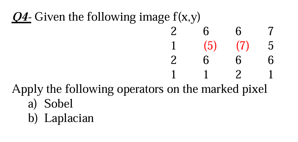
First, let's extract the
-
Neighborhood for Pixel (5):
-
Neighborhood for Pixel (7):
a) Sobel Operator
The Sobel operator calculates the gradient of the image using two kernels: one for horizontal changes (
The total magnitude is typically calculated as
1. Applying to Pixel (5):
-
: -
: -
Magnitude:
20
2. Applying to Pixel (7):
-
: -
: -
Magnitude:
1.41
b) Laplacian Operator
Got it! Thank you for the clarification. In some textbooks and courses, the "composite" Laplacian is indeed defined as adding the original image back to the standard Laplacian to sharpen it in one step. When you subtract a standard 4-neighbor Laplacian (with a
We'll calculate using the composite 4-neighbour
1. Applying to Pixel (5):
For the pixel at row 1, column 1, we look at its immediate top, bottom, left, and right neighbors.
-
Top neighbor: 6
-
Bottom neighbor: 6
-
Left neighbor: 1
-
Right neighbor: 7
-
Center pixel: 5
Calculation:
-
Sum of the 4 neighbors:
-
Multiply neighbors by
: -
Center multiplied by
: -
True Output:
5
2. Applying to Pixel (7):
For the pixel at row 1, column 2, we again look at its immediate 4-connected neighbors.
-
Top neighbor: 6
-
Bottom neighbor: 6
-
Left neighbor: 5 (this is the pixel we just calculated in the step above)
-
Right neighbor: 5
-
Center pixel: 7
Calculation:
Sum of the 4 neighbors:
Negate the sum:
Center multiplied by 5:
Output: