1. Piecewise-Linear Transformation Functions
These are functions that manipulate an image's contrast by mapping input pixel values to output pixel values using linear segments. The main types covered are contrast stretching, intensity-level slicing, and bit-plane slicing.
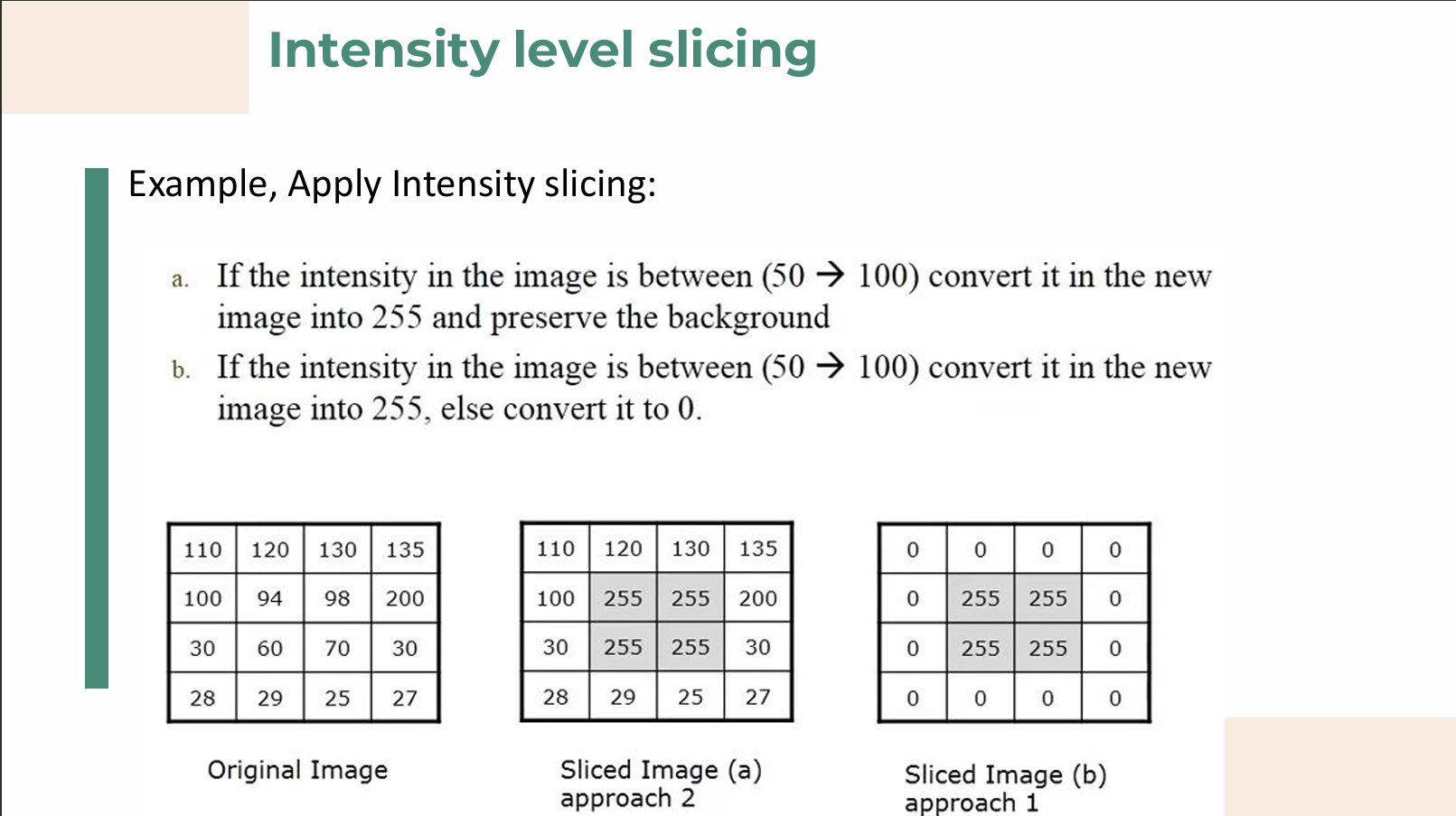
Intensity-Level Slicing
- Purpose: This technique highlights a specific range of grey levels within an image.
- Applications: It is mostly used for enhancing specific features, such as in satellite imagery or medical X-rays.
- Approach 1 (Binary Masking): Displays all values within the range of interest as one value (e.g., pure white or 255) and all other intensities as another value (e.g., pure black or 0).
- Approach 2 (Preserving Background): Brightens or darkens the desired range of intensities but leaves all other intensity levels in the image entirely unchanged, effectively preserving the original background.
Bit-Plane Slicing
- Concept: Instead of highlighting intensity ranges, this technique isolates particular bits of the pixel values to highlight interesting aspects of an image's structure.
- Structure: In a standard 256-level grayscale image, each pixel is composed of 8 bits (one byte). The image can be viewed as being composed of eight separate 1-bit planes.
- Plane 1 (LSB): Contains the lowest-order (least significant) bit of all pixels, which usually represents subtle details and noise.
- Plane 8 (MSB): Contains the highest-order (most significant) bit, which holds the majority of the visually significant data and structural information.
- Applications: It is highly useful for analyzing the relative importance of each bit (determining quantization adequacy) and for image compression, as reconstructing an image with fewer higher-order planes can still yield a visually acceptable result.
- Example: A pixel with a decimal value of 100 converts to the binary value
. The 3rd bit contributes a value of 4, the 6th bit contributes 32, and the 7th bit contributes 64 ( ).
2. Histogram Processing
A histogram is a fundamental graph indicating the number of times each gray level occurs, showing the overall distribution of grey levels in an image.
- Histogram Function: Defined as
.
- Variables:
represents the -th grey level, and is the total number of pixels in the image that have that specific grey level.
- Normalized Histogram: Defined as
, where is the total number of pixels in the image.
- Utility: This information is vital for applications like image compression and image segmentation.
Four Basic Image Types Based on Histograms
- Dark image: The histogram's components are concentrated strictly on the low (dark) side of the gray scale.
- Bright image: The histogram is heavily biased toward the high (light) side of the gray scale.
- Low-contrast image: The histogram is very narrow and centered toward the middle of the gray scale, lacking pure blacks and pure whites.
- High-contrast image: The histogram covers a broad range of the gray scale, with a relatively even distribution where very few vertical lines are significantly higher than the others.
3. Histogram Equalization
Histogram equalization is a mathematical technique used for adjusting image intensities to automatically enhance overall contrast. It works by mapping each pixel with level
The Core Formula
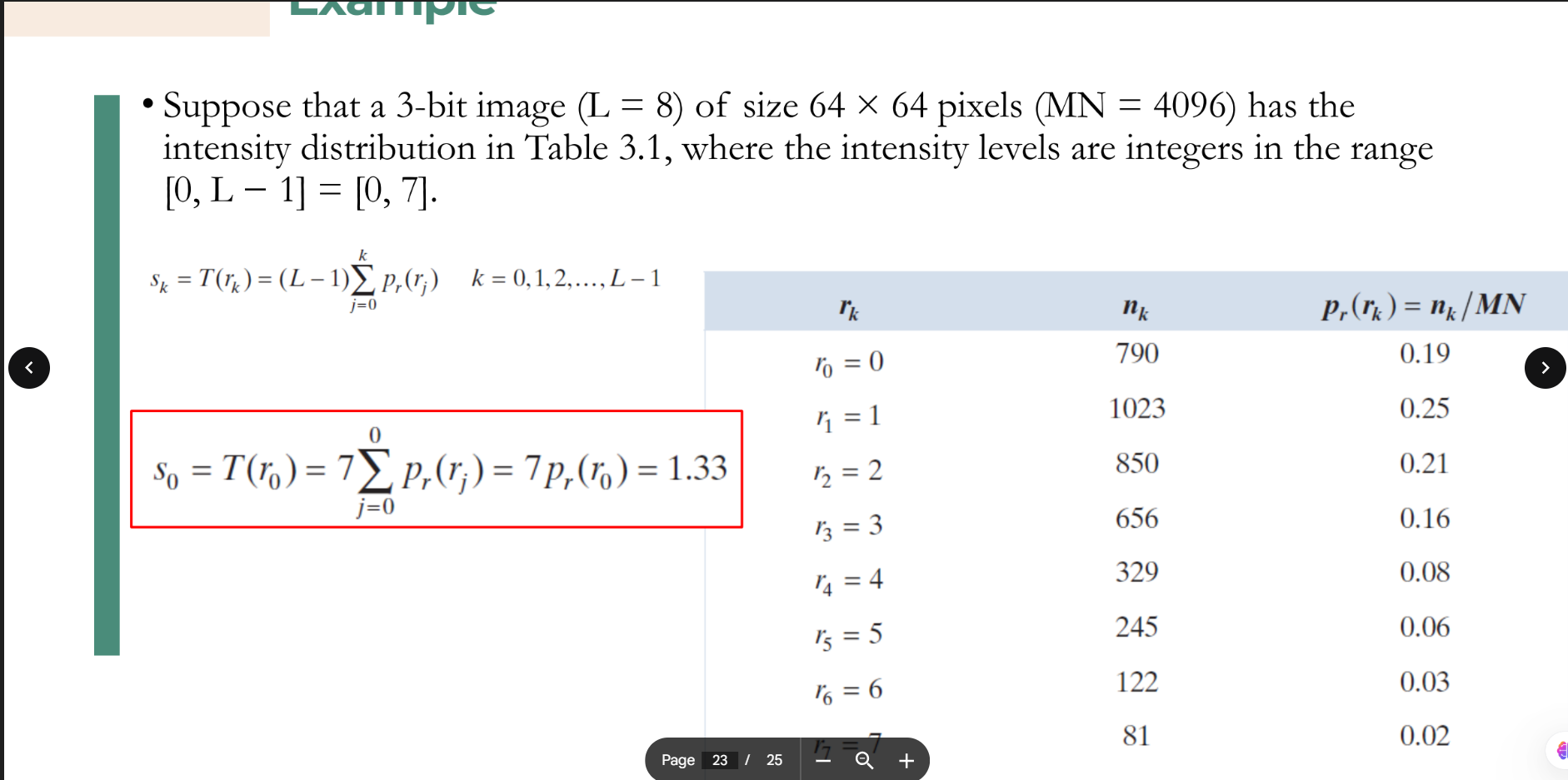
is the total number of possible intensity levels (e.g., 8 for a 3-bit image, 256 for an 8-bit image). . is the probability of occurrence of gray level .
Calculation Example
Suppose we have a 3-bit image (
-
Find Probabilities: Divide the count of pixels for each level (
) by the total pixels ( ) to get . - For
: . - For
: . - For
: .
- For
-
Apply Formula: Multiply the max intensity level (
, which is ) by the cumulative sum of probabilities up to that level. (rounds to 1). (rounds to 3). (rounds to 5).
-
Result: The original clustered gray levels (0, 1, 2) are now stretched out into new mapping values (1, 3, 5), creating a more uniform distribution and higher contrast.
Comparison between contrast stretching and histogram equalization
While both contrast stretching and histogram equalization are techniques used to improve the contrast of an image, they achieve this goal using entirely different mathematical approaches.
1. Contrast Stretching (Min-Max Stretching)
Contrast stretching is a linear (or piecewise-linear) transformation. It works by taking the narrow range of intensity values present in a low-contrast image and pulling them apart to fill the entire available dynamic range (e.g., from
- How it works: It identifies the darkest pixel (
) and the brightest pixel ( ) in the original image. It then applies a formula to map to absolute black ( ) and to absolute white ( ), scaling all the values in between linearly.
- The Result: The overall "shape" of the histogram remains the same; it is just stretched out horizontally like a rubber band.
2. Histogram Equalization
Histogram equalization is a non-linear transformation. Instead of just stretching the boundaries, it mathematically redistributes the pixel intensities so that they are as evenly distributed as possible across the entire range.
- How it works: It uses the image's cumulative distribution function (CDF). It finds the most frequent intensity values (the tallest peaks in the histogram) and spreads them out, while compressing the less frequent values.
- The Result: The original shape of the histogram is completely changed. The output image will have a roughly "flat" or uniform histogram where all gray levels occur with relatively similar frequency. This often reveals hidden details in very dark or very bright regions but can sometimes produce unnatural-looking results.
| Feature | Contrast Stretching | Histogram Equalization |
|---|---|---|
| Transformation Type | Linear (or Piecewise-Linear) | Non-linear |
| Primary Goal | Expands the existing range of pixels to fill the max/min limits. | Flattens the histogram to distribute pixels evenly. |
| Effect on Histogram | Keeps the relative shape, but makes it wider. | Completely alters the shape, aiming for a uniform distribution. |
| Visual Result | Usually looks natural, simply correcting "washed out" images. | Maximizes contrast heavily, which can sometimes look artificial or amplify noise. |
| Complexity | Computationally simple (relies on min/max values). | Computationally more complex (requires calculating probabilities and cumulative sums). |