#What "Are" Local Probabilistic Models and What is Their Purpose?
#**Q ** How do we handle large nodes with many variables?
#ICI Vs CSI
What "Are" Local Probabilistic Models and What is Their Purpose?
A Local Probabilistic Model is a mathematically efficient way to calculate the probability of a specific node in a network based on its parents, without having to write out every single possible combination of events.
In a standard network, the relationship between a child node and its parent nodes is defined by a Conditional Probability Table (CPT).
-
The Problem: If a node has
parents, and each parent can take values, the CPT needs rows. If a disease is caused by 10 different genetic markers, you would need a table with (1,024) probabilities. This is the curse of dimensionality. It requires too much memory, is impossible to learn from small datasets, and is extremely slow to compute. -
The Purpose/Solution: LPMs replace these massive, exhaustive tables with "local structures"—rules, functions, or trees that calculate the probability dynamically.
Why we use them: They drastically shrink the number of parameters you need. Instead of memorizing 1,024 separate probabilities, an LPM might only need 10 parameters to accurately predict the outcome. This makes networks faster, less memory-intensive, and much easier to train.
How LPMs Differ from Bayesian Networks
They don't actually differ; they are part of the same system. You can think of them in terms of "Macro" vs. "Micro" architecture.
-
Bayesian Networks (The Global Structure): A Bayesian Network is the overarching map. It shows the directed edges (arrows) between variables, mapping out the global dependencies (e.g., "Smoking" and "Genetics" point to "Lung Cancer").
-
Local Probabilistic Models (The Local Structure): An LPM is what lives inside that specific "Lung Cancer" node. Instead of a giant CPT detailing every combination of Smoking and Genetics, you plug an LPM inside that node to handle the math efficiently.
How LPMs Differ from Markovian Models
The difference here lies in the flow of causality and how relationships are defined.
-
Markov Models (Markov Networks / MRFs): These use undirected edges. They model symmetrical correlations rather than strict cause-and-effect. Because there are no "parents" or "children," they don't use conditional probabilities like
. Instead, they use "potential functions" (or factors) to measure how much certain variables agree with each other globally. -
Local Probabilistic Models: These belong strictly to directed models (like Bayesian Networks). They explicitly model directional causality. An LPM is highly specific: it is a formula designed solely to calculate
.
How LPMs are Exactly Related to Decision Trees
Decision trees are actually one of the primary types of Local Probabilistic Models. In this context, they are called Tree-CPDs (Tree Conditional Probability Distributions).
They are used to model a concept called Context-Specific Independence (CSI).
Imagine you are trying to predict if an entity will cough based on two parents: "Has a Cold" and "Entity Type" (Human or Robot).
-
In a standard CPT, you would map out all combinations: (Human, Cold), (Human, No Cold), (Robot, Cold), (Robot, No Cold).
-
In a Tree-CPD, you use a decision tree to route the logic.
-
The root of the tree asks: "Entity Type?"
-
If the branch goes to "Robot", the tree immediately hits a leaf node:
. -
Notice what happened: Because it's a robot, the tree never even asked if it had a cold.
-
The exact relationship: The decision tree acts as the LPM. By routing logic through branches, it snips off irrelevant variables depending on the "context" (e.g., if it's a robot, biological diseases become mathematically irrelevant). This bypasses the need for a massive table, effectively turning a decision tree into a highly efficient probability calculator inside a Bayesian Network.
Applying a Local Probabilistic Model (LPM) to this exact network does result in fewer numbers to calculate, though the savings are small here because the network itself is so tiny.
To understand how it applies, we have to look at where LPMs are useful. LPMs are designed to solve the problem of exponential growth in nodes that have multiple parents.
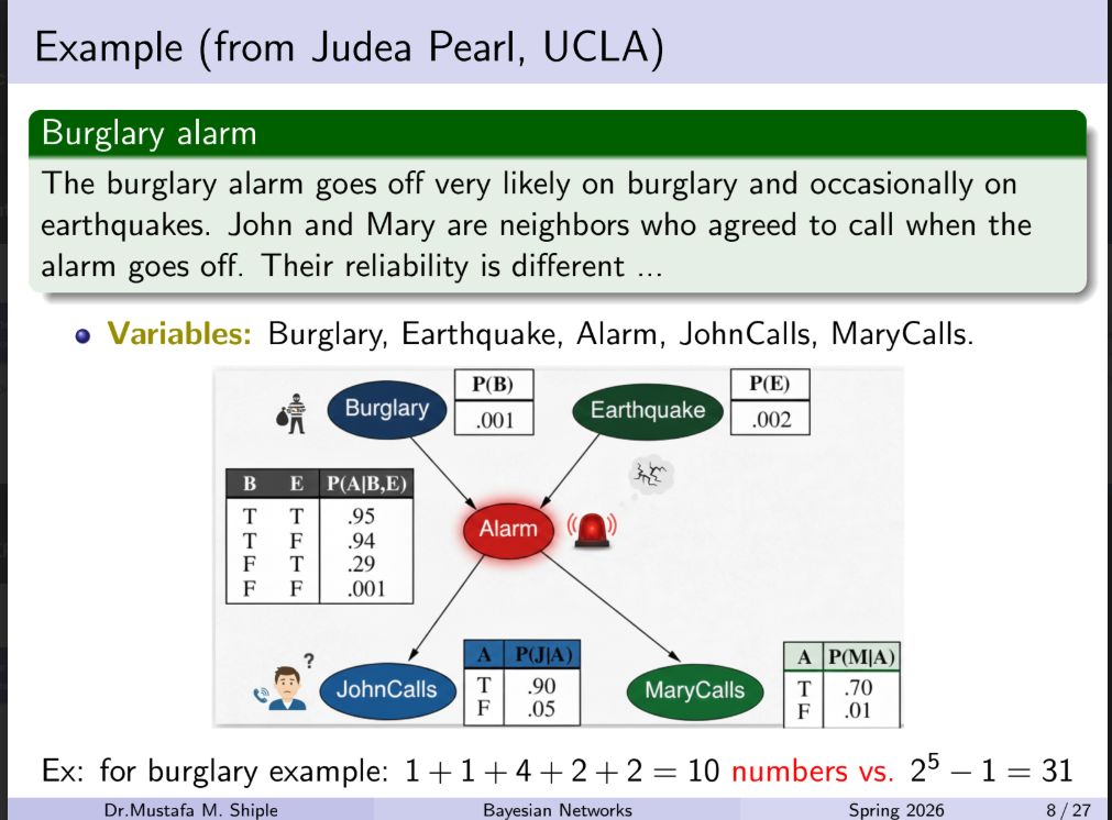
In the Burglary Alarm example, nodes like Burglary, Earthquake, JohnCalls, and MaryCalls only have zero or one parent. Their parameters are already at the absolute mathematical minimum (1 parameter for the priors, 2 parameters for the single-parent children).
The only target for an LPM in this network is the Alarm node, which has two parents (Burglary and Earthquake).
Here is how applying an LPM (specifically, the Noisy-OR model) changes the math:
1. The Standard Bayesian Network Approach
As shown in your image, the standard Conditional Probability Table (CPT) for the Alarm node lists every possible True/False combination of its parents.
-
Because it has 2 binary parents, the table requires 4 parameters (
). -
Total Network Parameters: 1 + 1 + 4 + 2 + 2 = 10
2. The Local Probabilistic Model (Noisy-OR) Approach
The Noisy-OR model operates on the principle of Independence of Causal Influence (ICI). It assumes that a Burglary and an Earthquake are independent mechanisms that can separately trigger the Alarm.
Instead of mapping out every combination, Noisy-OR only requires us to know the individual "strength" or "failure rate" of each cause.
To recreate the Alarm node using Noisy-OR, we only need parameters for:
-
The Burglary Trigger: The probability that a Burglary successfully triggers the alarm (or fails to).
-
The Earthquake Trigger: The probability that an Earthquake successfully triggers the alarm (or fails to).
-
The "Leak" Probability: The standard CPT shows a 0.001 chance the alarm goes off even if there is no burglary and no earthquake (a false alarm). In Noisy-OR, we add a single "leak" parameter to account for this background noise.
-
Using Noisy-OR, the
Alarmnode only requires 3 parameters instead of 4. -
New Total Network Parameters: 1 + 1 + 3 + 2 + 2 = 9
The Bigger Picture
In this specific example, the LPM reduces the total parameter count from 10 to 9.
While saving one single parameter doesn't sound impressive, imagine if the Alarm was connected to 10 different sensors (glass break, motion, door open, laser, etc.) instead of just two.
-
A standard CPT would require 1,024 parameters (
) just for the Alarm node. -
A Noisy-OR model would only require 11 parameters (1 for each of the 10 sensors, plus 1 leak parameter).
That is the true power of Local Probabilistic Models: they prevent the math from exploding when your network scales up.
Q: How do we handle large nodes with many variables?
A: By decomposing large nodes into sub-nodes, creating trees inside nodes, and reducing CPT sizes exponentially to simplify calculations.
This Q&A perfectly summarizes the core concept of Tree-CPDs and Independence of Causal Influence (ICI) from your lecture.
It is describing the exact mechanism of how Local Probabilistic Models (LPMs) solve the "Curse of Dimensionality."
1. "Large nodes with many variables"
In a standard Bayesian Network, a "node" is just a variable (like "Cough"). If that node has many "parent" variables pointing to it (e.g., "Cold", "Flu", "Smoking", "Asthma", "Dust"), it becomes a "large node."
The problem is that a standard Conditional Probability Table (CPT) requires a separate row for every single possible combination of those parents. If you have 10 binary parents, that one node requires a table with
2. "Creating trees inside nodes"
Normally, you look inside a node and see a massive, flat spreadsheet (the CPT). This strategy suggests throwing away the spreadsheet and replacing it with a decision tree (a Tree-CPD).
Instead of calculating every combination, the tree acts like a flowchart that routes logic based on Context-Specific Independence (CSI):
-
Root of the tree: "Is the patient Human or a Robot?"
-
Branch 1 (Robot): The tree immediately stops. The probability of a cough is 0. It completely ignores all the disease variables because they are irrelevant in this context.
-
Branch 2 (Human): The tree continues to ask about Cold, Flu, etc.
By putting a tree inside the node, you allow the model to skip over massive chunks of irrelevant data dynamically.
3. "Decomposing large nodes into sub-nodes"
This refers to how models like Noisy-OR are structurally built.
If 10 different diseases point directly to "Cough," the math gets tangled up because the standard CPT tries to calculate how all 10 interact with each other.
To fix this, we "decompose" the relationship by creating invisible, intermediate sub-nodes.
-
Instead of
, we model it as: . -
We do this for every disease.
-
Then, all those intermediate nodes feed into a single, simple logic gate (like a MAX or OR gate).
This isolates each parent variable. They no longer have to interact with each other in a giant table; they only interact with their own intermediate node.
4. "Reducing CPT sizes exponentially"
This is the ultimate payoff.
-
Without decomposition (Standard CPT): 10 parents =
= 1,024 parameters. (Exponential growth). -
With decomposition (Noisy-OR / Trees): 10 parents = 10 parameters (plus maybe a leak parameter). (Linear growth).
In short: The Q&A means that instead of using giant, exhaustive tables to calculate probabilities, we use smart, local logic structures (like flowcharts and isolated sub-nodes) to bypass unnecessary math and drastically shrink the computation size.
ICI Vs CSI
This is a complete comparison between Independence of Causal Influence (ICI) models and Context-Specific Independence (CSI) models, detailing their mechanics, limitations, and how they combine into a highly efficient hybrid approach.
1. Core Comparison: ICI vs. CSI
Both ICI and CSI are Local Probabilistic Models designed to solve the exponential parameter growth of standard Conditional Probability Tables (CPTs). However, they tackle the problem using completely different logical assumptions.
| Feature | Independence of Causal Influence (ICI) | Context-Specific Independence (CSI) |
|---|---|---|
| Core Logic | Accumulation: Multiple independent causes contribute to a single effect. | Routing: The relevance of some variables depends entirely on the state of another variable. |
| Model Types | Noisy-OR (Binary variables: "Does it happen?") Noisy-MAX (Ordinal variables: "To what degree does it happen?") |
Tree-CPDs (Decision trees built inside the node). |
| Visual Structure | A flat convergence of independent paths into a single logic gate (OR/MAX). | A branching flowchart or decision tree. |
| Parameter Scaling | Scales linearly with the number of parents ( |
Scales based on the number of leaves in the tree (paths that matter). |
2. Deep Dive: Limitations of Each Approach
While both models drastically reduce computation, they fail when applied to the wrong type of logical relationship.
Limitations of ICI (Noisy-OR & Noisy-MAX)
-
Inability to Handle "Switches" (Contexts): ICI assumes all parents are always potentially active causes. It cannot easily model a scenario where one parent acts as a master switch that completely negates the others. For example, if a machine is unplugged, the temperature sensors shouldn't just have a "low probability" of triggering a heat alarm—they should have a strictly
probability. ICI struggles to represent this absolute veto cleanly. -
The "No Synergy" Assumption: ICI strictly assumes that causes are independent. It fails if causes interact synergistically. For example, taking Drug A might have a
chance of causing side effects, and Drug B might have a chance. Noisy-OR assumes taking both yields roughly a chance. But in human biology, mixing those specific drugs might create a lethal chemical reaction with a chance of side effects. ICI cannot model this interaction.
Limitations of CSI (Tree-CPDs)
-
The "Accumulation" Blindspot: CSI is terrible at modeling scenarios where multiple variables do independently contribute to an effect. If a patient has 5 different independent diseases that can cause a fever, a Tree-CPD must branch out to ask about every single disease combination to calculate the final probability. In this scenario, the tree simply recreates the massive CPT, failing to reduce the parameter count.
-
Tree Depth: If many variables are relevant, the tree becomes overwhelmingly deep and complex, losing its computational advantage.
3. The Power of the Hybrid Approach
Because real-world scenarios usually involve both "switches" (contexts) and "accumulative triggers" (independent causes), combining them yields the most accurate and efficient model.
How it works:
You use a Tree-CPD as the outer framework to handle the logical routing and context-switching. Then, at the leaf nodes of that tree, instead of putting a single static probability, you embed an ICI model (like Noisy-OR) to handle the accumulative causes relevant to that specific context.
This gives you the best of both worlds: the strict logical rules of CSI and the linear parameter scaling of ICI.
4. Parameter Reduction Example
Let's look at a network to see exactly how each approach impacts the math.
The Scenario:
We have a node called Server Crash (
-
: Power Status (On/Off) - This is a context variable. -
: Four independent traffic spikes from different regions.
Standard Bayesian Network (Full CPT):
Because there are 5 binary parents, the CPT must account for every possible combination.
-
Calculation:
-
Total Parameters: 32
Approach A: Using CSI (Tree-CPD) Only
We build a tree. The root asks: "What is the Power Status (
-
If
: The server cannot crash from traffic. We hit a leaf node immediately ( ). That requires 1 parameter. -
If
: We now have to evaluate the traffic spikes. Because CSI cannot handle independent accumulation efficiently, it must branch out for every combination of , and . That requires leaves (16 parameters). -
Total Parameters:
17
Approach B: Using ICI (Noisy-OR) Only
We treat all 5 variables as independent causes with their own failure rates (
-
Calculation: 1 parameter for
, 4 parameters for the sensors, 1 leak parameter. -
Total Parameters: 6
-
The Flaw: While mathematically small, this is logically incorrect. It assumes the Power Status is just another "cause" of a crash, failing to recognize that if the power is off, the traffic spikes mathematically cannot cause a crash.
Approach C: The Hybrid Model
We use a tree for the context, and Noisy-OR for the accumulation.
-
The Tree: Root asks for Power Status (
). -
Branch 1 (
): Leaf node is a strict . (1 parameter). -
Branch 2 (
): Leaf node contains a Noisy-OR model for the 4 traffic spikes ( to ). This requires 4 trigger parameters plus 1 leak parameter (5 parameters).
- Total Parameters:
6
The Conclusion:
The Hybrid approach matches the extreme compression of the Noisy-OR model (reducing 32 parameters down to 6), while perfectly preserving the strict logical reality of the system that the Noisy-OR model alone would have missed.
Applying Local Probabilistic Concepts to Markovian Networks
In a Markov Network, because there is no cause-and-effect direction, you cannot isolate a "parent" and a "child." Instead, the network simplifies the math by grouping nodes that heavily interact with each other into isolated clusters.
Here is a detailed breakdown of exactly how this Markovian simplification works, mirroring the logic of your lecture notes.
1. The Anatomy of Simplification: Cliques vs. Groups
To break down a massive undirected network, you have to find the boundaries of interaction. This is done by identifying cliques.
-
A Group: This is a loose collection of nodes. If Node A talks to Node B, and Node B talks to Node C, they are a group. But because A doesn't talk directly to C, you can't easily isolate them as a single mathematical unit.
-
A Clique: This is a strictly defined, fully connected sub-graph. Every single node inside a clique has a direct connection to every other node in that clique. Because they are all "talking" directly to each other, they share high similarity and dependencies, making them the perfect candidate to act as a localized, independent mathematical unit.
2. Clique-Based Network Decomposition
In a Bayesian Network, LPMs decompose large nodes by creating invisible sub-nodes (like the independent triggers in Noisy-OR).
In a Markov Network, decomposition works by literally slicing the global network apart into its maximal cliques.
-
If you have a giant network of 100 nodes, trying to calculate the joint probability of the entire board at once is mathematically impossible.
-
Instead, you find the cliques. If you can divide the network into overlapping cliques (e.g., Sub-network 1 and Sub-network 2, connected by one shared node), you can process them completely independently.
3. The Quantitative Payoff (The 6-Node Example)
This is where the massive reduction in parameters happens, directly mirroring the mathematical savings of something like a Noisy-OR model.
Imagine a network of 6 binary nodes (variables that can be True or False).
-
Without Decomposition (The Global View): To process the whole network at once, you must calculate every possible combination of those 6 nodes interacting. That requires 2^6 = 64 distinct records or states.
-
With Decomposition (The Local View): You identify that these 6 nodes actually form two distinct cliques of 3 nodes each (perhaps joined by a single common node in the middle).
-
Instead of one giant table of 64 calculations, you calculate the states for Clique 1 (2^3 = 8) and Clique 2 (2^3 = 8).
-
You have immediately reduced the computational load from 64 distinct combinations down to just 16.
-
4. Similarity and Relative Probabilities
Your notes mention that by "assuming similarity within them, the number of distinct combinations reduces drastically to a few representative cases."
This is a massive advantage in Markov Networks. If the nodes inside a clique represent similar entities (like neighboring pixels in an image, or similar words in a sentence), you don't even need to calculate completely separate probabilities for them.
You can use the exact same feature weights (multiplying probabilities of similar nodes) across the board. Instead of counting absolute occurrences, the network calculates relative probabilities (how likely one state is compared to another within that specific, isolated clique), making the model highly scalable no matter how large the overall network gets.