Q1

There appears to be a typo in the diagram. The bottom arrow originating from $X_2$ and pointing to $H_3$ is labeled as $W_{X2-H1}=0.2$. Based on the network's structure, I will logically assume this represents $W_{X2-H3}=0.2$.

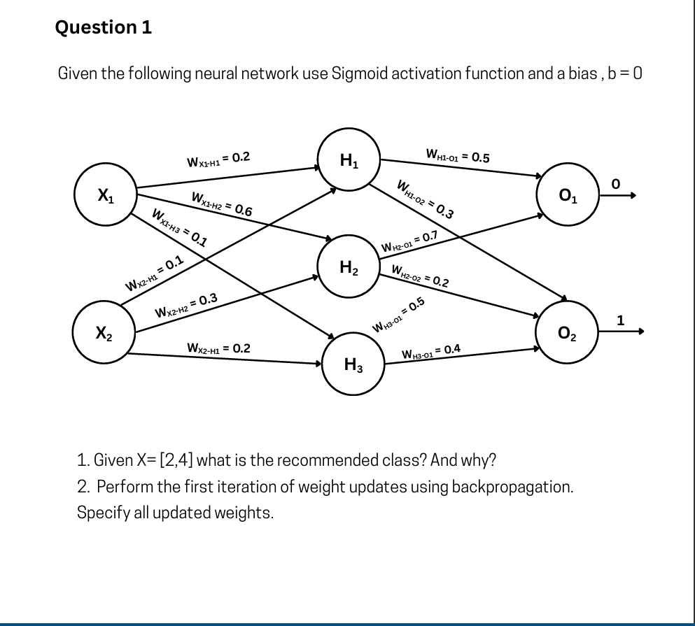
1. Given X = [2,4] what is the recommended class? And why?

To find the recommended class, we need to perform a forward pass through the network using the given inputs ($X_1=2$, $X_2=4$), a bias of 0, and the Sigmoid activation function: $\sigma (z)=\frac{1}{1+e^{-z}}$.

Step A: Calculate Hidden Layer Activations ($H_1,H_2,H_3$)

First, we find the weighted sum ($Z$) for each hidden node, then apply the Sigmoid function.

• For $H_1$:

  $$Z_{H1}=(X_1\cdot W_{X1-H1})+(X_2\cdot W_{X2-H1})+b$$$$Z_{H1}=(2\cdot 0.2)+(4\cdot 0.1)+0=0.4+0.4=0.8$$$$H_1=\sigma (0.8)=\frac{1}{1+e^{-0.8}}\approx \mathbf{0.690}$$

• For $H_2$:

  $$Z_{H2}=(X_1\cdot W_{X1-H2})+(X_2\cdot W_{X2-H2})+b$$$$Z_{H2}=(2\cdot 0.6)+(4\cdot 0.3)+0=1.2+1.2=2.4$$$$H_2=\sigma (2.4)=\frac{1}{1+e^{-2.4}}\approx \mathbf{0.917}$$

• For $H_3$:

  $$Z_{H3}=(X_1\cdot W_{X1-H3})+(X_2\cdot W_{X2-H3})+b$$$$Z_{H3}=(2\cdot 0.1)+(4\cdot 0.2)+0=0.2+0.8=1.0$$$$H_3=\sigma (1.0)=\frac{1}{1+e^{-1.0}}\approx \mathbf{0.731}$$

Step B: Calculate Output Layer Activations ($O_1,O_2$)

Now, we use the hidden layer activations to compute the final outputs.

• For $O_1$ (Class 0):

  $$Z_{O1}=(H_1\cdot W_{H1-O1})+(H_2\cdot W_{H2-O1})+(H_3\cdot W_{H3-O1})+b$$$$Z_{O1}=(0.690\cdot 0.5)+(0.917\cdot 0.7)+(0.731\cdot 0.5)+0$$$$Z_{O1}=0.345+0.6419+0.3655=1.3524$$$$O_1=\sigma (1.3524)=\frac{1}{1+e^{-1.3524}}\approx \mathbf{0.794}$$

• For $O_2$ (Class 1):

  $$Z_{O2}=(H_1\cdot W_{H1-O2})+(H_2\cdot W_{H2-O2})+(H_3\cdot W_{H3-O2})+b$$$$Z_{O2}=(0.690\cdot 0.3)+(0.917\cdot 0.2)+(0.731\cdot 0.4)+0$$$$Z_{O2}=0.207+0.1834+0.2924=0.6828$$$$O_2=\sigma (0.6828)=\frac{1}{1+e^{-0.6828}}\approx \mathbf{0.664}$$

Conclusion:

The recommended class is Class 0.

Why: The calculated activation for the $O_1$ node (0.794), which corresponds to Class 0, is greater than the activation for the $O_2$ node (0.664), which corresponds to Class 1.

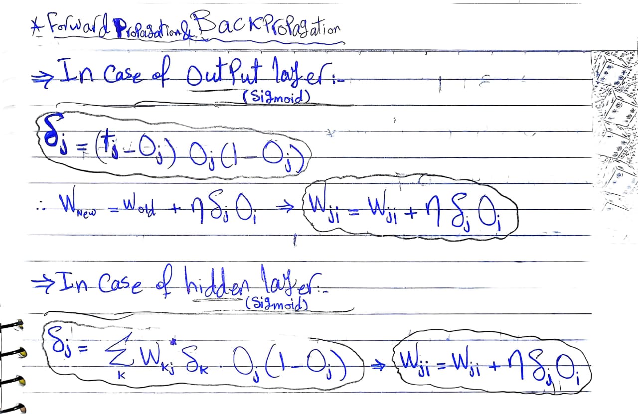
2. Perform the first iteration of weight updates using backpropagation. Specify all updated weights.

To perform a mathematical weight update via backpropagation, two critical pieces of information are missing from the problem prompt:

1. The True Target Labels ($Y$): We need to know what the network should have predicted for the input $X=[2,4]$ to calculate the loss/error margin.

2. The Learning Rate ($\eta$): We need the hyperparameter that determines the step size of the weight updates.

How to proceed:

If you can provide the target labels and the learning rate expected by your professor or assignment, I can complete the backpropagation calculations for you.

As a reference, once you have those values, the update for a weight connecting the hidden layer to the output layer (assuming Mean Squared Error loss) would follow this formula:

Setup & Values from the Forward Pass

• Learning Rate ($\eta$): 0.1

• Target ($T$): The previous recommended class was Class 0. The opposite is Class 1. Therefore, the target values for the output nodes are: $T_1=0$ (for $O_1$) and $T_2=1$ (for $O_2$).

• Inputs: $X_1=2$, $X_2=4$

• Cached Forward Pass Activations (rounded to 4 decimal places for accuracy):

  • $H_1=0.6900$, $H_2=0.9168$, $H_3=0.7311$

  • $O_1=0.7945$, $O_2=0.6644$

(Note: We will use the standard Mean Squared Error loss derivative for the Sigmoid activation function: $\delta =(Output-Target)\cdot Output\cdot (1-Output)$)

Step 1: Calculate the Output Layer Errors (${\delta }_O$)

• For $O_1$ (Target $T_1=0$):

  $${\delta }_{O1}=(O_1-T_1)\cdot O_1\cdot (1-O_1)$$$${\delta }_{O1}=(0.7945-0)\cdot 0.7945\cdot (1-0.7945)$$$${\delta }_{O1}=0.7945\cdot 0.7945\cdot 0.2055\approx \mathbf{0.1297}$$

• For $O_2$ (Target $T_2=1$):

  $${\delta }_{O2}=(O_2-T_2)\cdot O_2\cdot (1-O_2)$$$${\delta }_{O2}=(0.6644-1)\cdot 0.6644\cdot (1-0.6644)$$$${\delta }_{O2}=(-0.3356)\cdot 0.6644\cdot 0.3356\approx \mathbf{-}\mathbf{0.0748}$$

Step 2: Update the Output Layer Weights

The weight update formula is: $W_{new}=W_{old}-\eta \cdot {\delta }_O\cdot H$

• $W_{H1-O1}=0.5-(0.1\cdot 0.1297\cdot 0.6900)=0.5-0.0089=\mathbf{0.4911}$

• $W_{H2-O1}=0.7-(0.1\cdot 0.1297\cdot 0.9168)=0.7-0.0119=\mathbf{0.6881}$

• $W_{H3-O1}=0.5-(0.1\cdot 0.1297\cdot 0.7311)=0.5-0.0095=\mathbf{0.4905}$

• $W_{H1-O2}=0.3-(0.1\cdot -0.0748\cdot 0.6900)=0.3+0.0052=\mathbf{0.3052}$

• $W_{H2-O2}=0.2-(0.1\cdot -0.0748\cdot 0.9168)=0.2+0.0069=\mathbf{0.2069}$

• $W_{H3-O2}=0.4-(0.1\cdot -0.0748\cdot 0.7311)=0.4+0.0055=\mathbf{0.4055}$

Step 3: Calculate the Hidden Layer Errors (${\delta }_H$)

To calculate the error for the hidden nodes, we backpropagate the output errors using the original weights before they were updated.

Formula: ${\delta }_H=(\sum {\delta }_O\cdot W_{new})\cdot H\cdot (1-H)$

• For $H_1$:

  $${\delta }_{H1}=({\delta }_{O1}\cdot W_{H1-O1}+{\delta }_{O2}\cdot W_{H1-O2})\cdot H_1\cdot (1-H_1)$$$${\delta }_{H1}=(0.1297\cdot 0.5+(-0.0748)\cdot 0.3)\cdot 0.6900\cdot (1-0.6900)$$$${\delta }_{H1}=(0.06485-0.02244)\cdot 0.2139=0.04241\cdot 0.2139\approx \mathbf{0.0091}$$

• For $H_2$:

  $${\delta }_{H2}=({\delta }_{O1}\cdot W_{H2-O1}+{\delta }_{O2}\cdot W_{H2-O2})\cdot H_2\cdot (1-H_2)$$$${\delta }_{H2}=(0.1297\cdot 0.7+(-0.0748)\cdot 0.2)\cdot 0.9168\cdot (1-0.9168)$$$${\delta }_{H2}=(0.09079-0.01496)\cdot 0.0763=0.07583\cdot 0.0763\approx \mathbf{0.0058}$$

• For $H_3$:

  $${\delta }_{H3}=({\delta }_{O1}\cdot W_{H3-O1}+{\delta }_{O2}\cdot W_{H3-O2})\cdot H_3\cdot (1-H_3)$$$${\delta }_{H3}=(0.1297\cdot 0.5+(-0.0748)\cdot 0.4)\cdot 0.7311\cdot (1-0.7311)$$$${\delta }_{H3}=(0.06485-0.02992)\cdot 0.1966=0.03493\cdot 0.1966\approx \mathbf{0.0069}$$

Step 4: Update the Hidden Layer Weights

The weight update formula is: $W_{new}=W_{old}-\eta \cdot {\delta }_H\cdot X$

• $W_{X1-H1}=0.2-(0.1\cdot 0.0091\cdot 2)=0.2-0.0018=\mathbf{0.1982}$

• $W_{X2-H1}=0.1-(0.1\cdot 0.0091\cdot 4)=0.1-0.0036=\mathbf{0.0964}$

• $W_{X1-H2}=0.6-(0.1\cdot 0.0058\cdot 2)=0.6-0.0012=\mathbf{0.5988}$

• $W_{X2-H2}=0.3-(0.1\cdot 0.0058\cdot 4)=0.3-0.0023=\mathbf{0.2977}$

• $W_{X1-H3}=0.1-(0.1\cdot 0.0069\cdot 2)=0.1-0.0014=\mathbf{0.0986}$

• $W_{X2-H3}=0.2-(0.1\cdot 0.0069\cdot 4)=0.2-0.0028=\mathbf{0.1972}$ (Using the assumed correction from earlier that the bottom-most arrow is $W_{X2-H3}$)

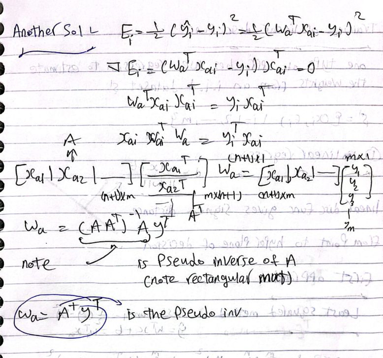
Q2: Derive the weight equation of Minimum sum squared errors.

Q3

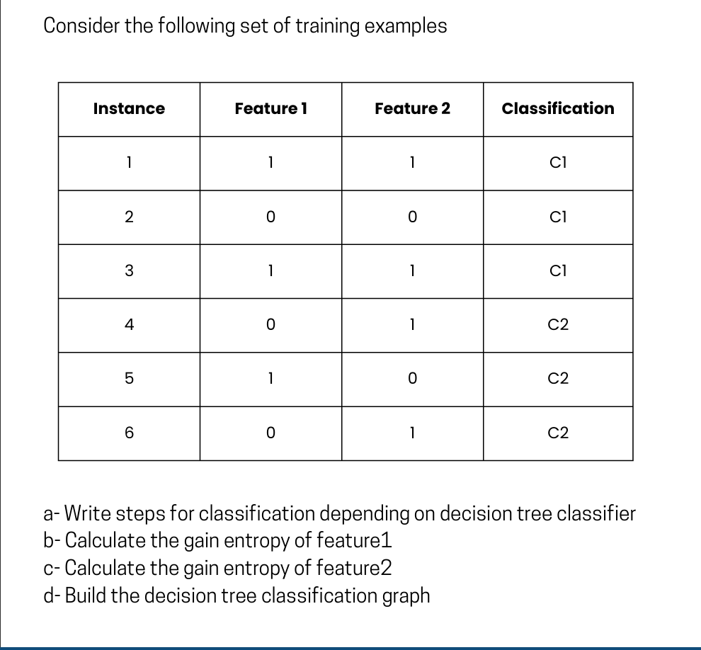
a- Steps for classification depending on decision tree classifier

To build a decision tree (specifically using the ID3 algorithm which relies on Information Gain), you follow these standard steps:

1. Calculate the Entropy of the target dataset: Determine the uncertainty of the entire dataset based on the class labels.

2. Calculate the Entropy for each feature: For every feature, calculate the entropy of its individual branches (values) and then compute the weighted average entropy for that feature.

3. Calculate Information Gain: Subtract the weighted entropy of each feature from the target dataset's total entropy.

4. Select the Root Node: Choose the feature with the highest Information Gain to split the dataset.

5. Repeat for Child Nodes: Recursively apply steps 1-4 to the subsets of data created by the split. Stop when a subset is pure (contains only one class) or when no more features are left to split.

Initial Calculation: Parent Entropy

Before calculating the gain for specific features, we must find the total entropy of the dataset, $E(S)$.

• Total instances ($N$) = 6

• Class C1 count = 3

• Class C2 count = 3

b- Calculate the gain entropy of Feature 1

First, we analyze the splits if we use Feature 1:

• If Feature 1 = 0: Instances {2, 4, 6} (Total = 3)

  • C1 count = 1 (Instance 2)

  • C2 count = 2 (Instances 4, 6)

  • $$E(F1=0)=-\left(\frac{1}{3}\right){\log }_2\left(\frac{1}{3}\right)-\left(\frac{2}{3}\right){\log }_2\left(\frac{2}{3}\right)\approx 0.918$$

• If Feature 1 = 1: Instances {1, 3, 5} (Total = 3)

  • C1 count = 2 (Instances 1, 3)

  • C2 count = 1 (Instance 5)

  • $$E(F1=1)=-\left(\frac{2}{3}\right){\log }_2\left(\frac{2}{3}\right)-\left(\frac{1}{3}\right){\log }_2\left(\frac{1}{3}\right)\approx 0.918$$

Now, calculate the weighted entropy for Feature 1, $E(S|F1)$:

Finally, calculate Information Gain:

c- Calculate the gain entropy of Feature 2

Next, we analyze the splits if we use Feature 2:

• If Feature 2 = 0: Instances {2, 5} (Total = 2)

  • C1 count = 1 (Instance 2)

  • C2 count = 1 (Instance 5)

  • $$E(F2=0)=-\left(\frac{1}{2}\right){\log }_2\left(\frac{1}{2}\right)-\left(\frac{1}{2}\right){\log }_2\left(\frac{1}{2}\right)=1.0$$

• If Feature 2 = 1: Instances {1, 3, 4, 6} (Total = 4)

  • C1 count = 2 (Instances 1, 3)

  • C2 count = 2 (Instances 4, 6)

  • $$E(F2=1)=-\left(\frac{2}{4}\right){\log }_2\left(\frac{2}{4}\right)-\left(\frac{2}{4}\right){\log }_2\left(\frac{2}{4}\right)=1.0$$

Now, calculate the weighted entropy for Feature 2, $E(S|F2)$:

Finally, calculate Information Gain:

d- Build the decision tree classification graph

Since Feature 1 has the higher Information Gain ($0.082>0.0$), it becomes the root node.

Because neither subset is perfectly pure after the first split, we apply Feature 2 to the resulting branches to complete the classification:

• If $F1=0$, looking at the dataset, $F2=0$ results purely in C1, and $F2=1$ results purely in C2.

• If $F1=1$, looking at the dataset, $F2=0$ results purely in C2, and $F2=1$ results purely in C1.

Here is the resulting decision tree structure:

Plaintext

          [Feature 1]
           /       \
        (0)         (1)
        /             \
  [Feature 2]     [Feature 2]
    /     \         /     \
  (0)     (1)     (0)     (1)
  /         \     /         \
[C1]       [C2] [C2]       [C1]

Q4

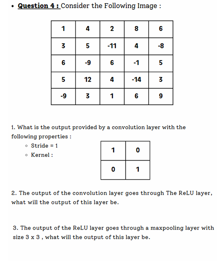
1. What is the output provided by a convolution layer?

We have a $5\times 5$ input image and a $2\times 2$ kernel with a stride of 1.

The output size will be: $\frac{5-2}{1}+1=4\times 4$. (Assuming zero padding)

The kernel is essentially an identity matrix:

This means that for every $2\times 2$ window the kernel slides over, we multiply the elements element-wise and sum them. Because of the 0s in the kernel, this operation simplifies to adding the top-left and bottom-right elements of the current $2\times 2$ window.

• Row 1 Calculations:

  • Window 1 (cols 1-2): $(1\cdot 1)+(5\cdot 1)=6$

  • Window 2 (cols 2-3): $(4\cdot 1)+(-11\cdot 1)=-7$

  • Window 3 (cols 3-4): $(2\cdot 1)+(4\cdot 1)=6$

  • Window 4 (cols 4-5): $(8\cdot 1)+(-8\cdot 1)=0$

Following this sliding window process across the entire matrix gives us the following output feature map:

2. The output of the convolution layer goes through The ReLU layer, what will the output of this layer be?

The Rectified Linear Unit (ReLU) activation function sets all negative values to zero while keeping positive values unchanged: $f(x)=max(0,x)$.

Applying this to our $4\times 4$ feature map from step 1:

3. The output of the ReLU layer goes through a maxpooling layer with size $3\times 3$, what will the output of this layer be?

Max pooling extracts the maximum value from the window. The problem does not explicitly state the stride for the pooling layer. When dealing with a $4\times 4$ matrix and a $3\times 3$ pool size, a standard default assumption in academic contexts (when stride isn't given) is a stride of 1, allowing the windows to overlap to capture edge features.

(Note: If the stride were 3, only one $3\times 3$ window would fit without padding, resulting in a single value of 18. Assuming a stride of 1 yields a $2\times 2$ output.)

Using a $3\times 3$ window with a stride of 1 on the ReLU output:

• Top-Left Window: The max value in the upper $3\times 3$ quadrant is $\mathbf{18}$.

• Top-Right Window: The max value in the upper right $3\times 3$ quadrant is $\mathbf{11}$.

• Bottom-Left Window: The max value in the lower left $3\times 3$ quadrant is $\mathbf{18}$.

• Bottom-Right Window: The max value in the lower right $3\times 3$ quadrant is $\mathbf{13}$.

Final Output Matrix:

Q5

1. Difference between Bagging and Boosting

Both are ensemble learning techniques used to improve model performance, but they operate differently:

2. Assumptions of Linear Regression

For a linear regression model to be valid and reliable, it relies on four main assumptions (often remembered by the acronym LINE), plus one regarding features:

• Linearity: The relationship between the independent variables (X) and the mean of the dependent variable (Y) is strictly linear.

• Independence: The observations (and thus the residuals) are independent of one another. There is no hidden autocorrelation.

• Normality of Residuals: The error terms (residuals) of the model are normally distributed.

• Equal Variance (Homoscedasticity): The variance of the residuals remains constant across all values of the independent variables (the spread of errors doesn't fan out or funnel in).

• No Multicollinearity: The independent variables should not be highly correlated with each other.

3. Importance of Data Normalization

Data normalization (scaling numerical features to a standard range, like 0 to 1, or standardizing them to have a mean of 0 and a variance of 1) is critical for several reasons:

• Equal Feature Weighting: It prevents features with naturally larger numerical ranges (e.g., salary in the thousands) from dominating features with smaller ranges (e.g., age in decades) when using distance-based algorithms like KNN or K-Means.

• Faster Convergence: In optimization algorithms like Gradient Descent (used in Neural Networks and Logistic Regression), normalized data creates a smoother, more symmetrical error landscape, allowing the model to converge to the minimum much faster.

• Numerical Stability: It prevents issues like vanishing or exploding gradients and floating-point overflow during computation in deep learning.

4. Convolutional Layer Calculations

Here are the calculations based on your provided parameters:

• Input ($W_{in}\times H_{in}\times D_{in}$): $224\times 224\times 3$

• Filters ($N$): 128

• Filter Size ($K$): $7\times 7$ (Depth is 3, matching the input)

• Stride ($S$): 3

• Padding ($P$): 2

a. Calculate the width and height of the output feature maps:

We use the standard dimension formula: $W_{out}=\lfloor \frac{W_{in}-K+2P}{S}\rfloor +1$

Because the input is square ($224\times 224$), the height will be the same.

• Output Width and Height: $\mathbf{74}\times \mathbf{74}$ (The full output volume is $74\times 74\times 128$).

b. Determine the total number of units (neurons) in the output:

The total number of units is the volume of the output feature map (Width $\times$ Height $\times$ Number of Filters).

• $\text{Total Units}=74\times 74\times 128$

• $\text{Total Units}=5,476\times 128=\mathbf{700}\mathbf{,}\mathbf{928}\text{ neurons}$

c. Compute the total number of learnable parameters:

Each filter has weights corresponding to its volume, plus exactly one bias term. We then multiply by the total number of filters.

• $\text{Weights per filter}=K\times K\times D_{in}=7\times 7\times 3=147$

• $\text{Bias per filter}=1$

• $\text{Total parameters per filter}=147+1=148$

• $\text{Total parameters for the layer}=148\times 128\text{ filters}=\mathbf{18}\mathbf{,}\mathbf{944}\text{ parameters}$