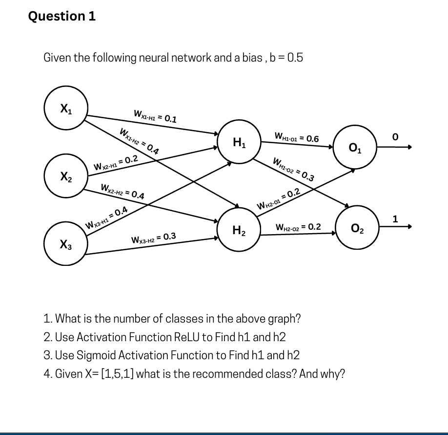
Q1

To solve questions 2 and 3, we need to use the input values provided in question 4: $X=[1,5,1]$, where $X_1=1$, $X_2=5$, and $X_3=1$. We will also apply the given bias $b=0.5$ to each node.

First, let's calculate the pre-activation values (the weighted sum plus bias) for the hidden nodes $H_1$ and $H_2$. We'll call these $Z_{H1}$ and $Z_{H2}$.

1. What is the number of classes in the above graph?

There are 2 classes.

The output layer consists of two nodes ($O_1$ and $O_2$), and the arrows pointing outward denote the respective class labels: 0 and 1.

2. Use Activation Function ReLU to Find $h_1$ and $h_2$

The ReLU (Rectified Linear Unit) activation function outputs the input directly if it is positive, otherwise, it outputs zero: $f(z)=max(0,z)$.

• $h_1=max(0,2.0)=\mathbf{2.0}$

• $h_2=max(0,3.2)=\mathbf{3.2}$

3. Use Sigmoid Activation Function to Find $h_1$ and $h_2$

The Sigmoid activation function is defined as: $\sigma (z)=\frac{1}{1+e^{-z}}$.

• $h_1=\frac{1}{1+e^{-2.0}}\approx \frac{1}{1+0.135}\approx \mathbf{0.88}$

• $h_2=\frac{1}{1+e^{-3.2}}\approx \frac{1}{1+0.041}\approx \mathbf{0.96}$

4. Given $X=[1,5,1]$ what is the recommended class? And why?

To find the recommended class, we need to compute the final values for the output nodes $O_1$ and $O_2$. We will use the standard practice of carrying forward the ReLU activations ($h_1=2.0$, $h_2=3.2$) from step 2, as ReLU is standard for hidden layers, and apply the given bias $b=0.5$.

Let's calculate the pre-activation outputs for $O_1$ (Class 0) and $O_2$ (Class 1):

Conclusion:

The recommended class is Class 0.

Why: Because the calculated value for the $O_1$ node ($2.34$) is greater than the value for the $O_2$ node ($1.74$). In classification networks, the node with the highest activation determines the predicted class. (Note: Using the Sigmoid values from step 3 would also result in $O_1$ having a higher value than $O_2$, leading to the exact same classification).

Q2

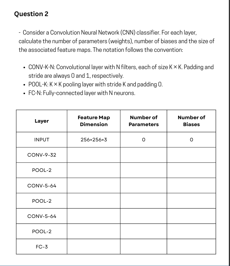
Completed Table

Formulas Used

The problem explicitly asks to separate the "Number of Parameters (Weights)" from the "Number of Biases".

1. Feature Map Dimension:

• Convolution Layer: $W_{out}=\frac{W_{in}-K+2P}{S}+1$

  • Given $P=0$ and $S=1$, this simplifies to: $W_{out}=W_{in}-K+1$

• Pooling Layer: $W_{out}=\frac{W_{in}-K}{S}+1$

  • Given stride $S=K$, this simplifies to: $W_{out}=\frac{W_{in}}{K}$

2. Number of Parameters (Weights):

• Convolution Layer: $(K\times K\times C_{in})\times C_{out}$ (where $C_{in}$ is input channels/depth, $C_{out}$ is number of filters $N$).

• Pooling Layer: $0$ (Pooling has no learnable weights).

• Fully-Connected Layer: $Feature{s}_{in}\times Neuron{s}_{out}$ (Requires flattening the previous layer's output).

3. Number of Biases:

• Convolution Layer: 1 bias per filter = $N$

• Fully-Connected Layer: 1 bias per neuron = $N$

Step-by-Step Breakdown

1. CONV-9-32

• Dimension: $W_{out}=256-9+1=248$. The depth becomes 32 (number of filters). $\to \mathbf{248}\times \mathbf{248}\times \mathbf{32}$

• Weights: $9\times 9\times 3(\text{input depth})\times 32=81\times 3\times 32=\mathbf{7}\mathbf{,}\mathbf{776}$

• Biases: $\mathbf{32}$

2. POOL-2

• Dimension: $W_{out}=\frac{248}{2}=124$. Depth remains unchanged. $\to \mathbf{124}\times \mathbf{124}\times \mathbf{32}$

• Weights & Biases: $\mathbf{0}$ (Pooling layers only perform aggregation, e.g., max or average).

3. CONV-5-64

• Dimension: $W_{out}=124-5+1=120$. Depth becomes 64. $\to \mathbf{120}\times \mathbf{120}\times \mathbf{64}$

• Weights: $5\times 5\times 32(\text{input depth})\times 64=25\times 32\times 64=\mathbf{51}\mathbf{,}\mathbf{200}$

• Biases: $\mathbf{64}$

4. POOL-2

• Dimension: $W_{out}=\frac{120}{2}=60$. Depth remains 64. $\to \mathbf{60}\times \mathbf{60}\times \mathbf{64}$

• Weights & Biases: $\mathbf{0}$

5. CONV-5-64

• Dimension: $W_{out}=60-5+1=56$. Depth remains 64. $\to \mathbf{56}\times \mathbf{56}\times \mathbf{64}$

• Weights: $5\times 5\times 64(\text{input depth})\times 64=25\times 64\times 64=\mathbf{102}\mathbf{,}\mathbf{400}$

• Biases: $\mathbf{64}$

6. POOL-2

• Dimension: $W_{out}=\frac{56}{2}=28$. Depth remains 64. $\to \mathbf{28}\times \mathbf{28}\times \mathbf{64}$

• Weights & Biases: $\mathbf{0}$

7. FC-3

• Note: Before passing data to a Fully-Connected layer, the 3D output of the previous layer must be flattened into a 1D vector. * Flattened Size: $28\times 28\times 64=\mathbf{50}\mathbf{,}\mathbf{176}$ features.

• Dimension: The output is simply a 1D array representing the 3 classes. $\to \mathbf{3}$

• Weights: $50,176(\text{flattened inputs})\times 3(\text{neurons})=\mathbf{150}\mathbf{,}\mathbf{528}$

• Biases: $\mathbf{3}$

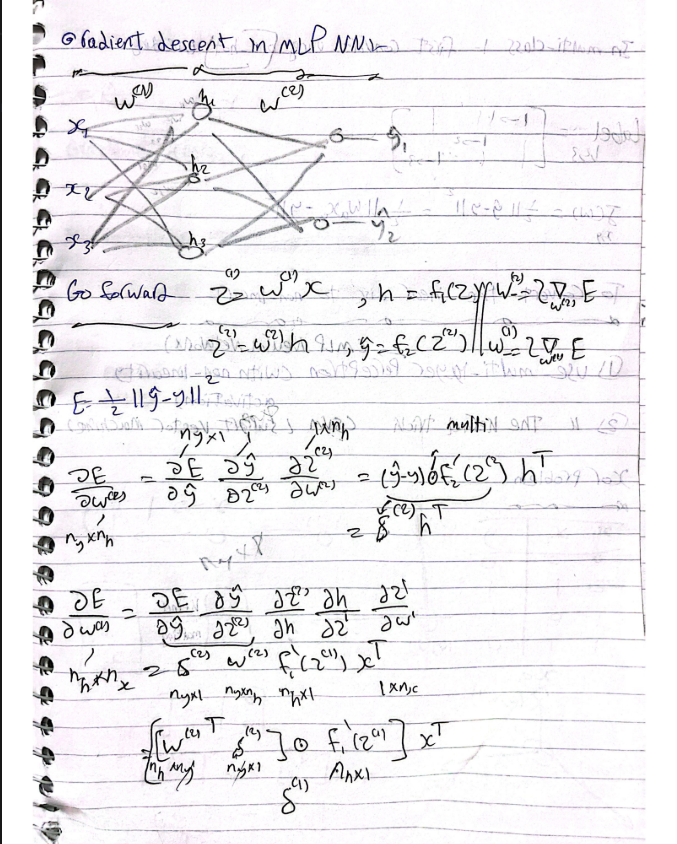
Q3

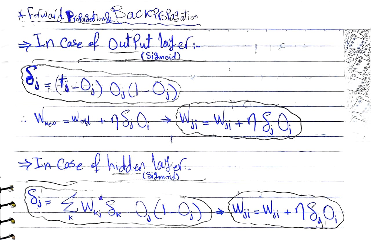
Proof

Q4: MCQ

Question 1

In K-Nearest Neighbors (KNN), what is the effect of choosing a very small value for 'K' (e.g., K=1)?

• Correct Answer: A. The model becomes more prone to overfitting the training data.

• Explanation: When K=1, the model strictly assigns the class of the single closest data point. This makes the decision boundary highly complex and jagged because it reacts to every single piece of noise or outlier in the training data. This high variance and low bias scenario is the classic definition of overfitting.

Question 2

What is a potential consequence of setting the learning rate (η) too high in gradient descent?

• Correct Answer: B. The gradient descent algorithm will oscillate around the minimum without converging, overshooting the optimal values.

• Explanation: The learning rate determines the size of the steps the algorithm takes down the error gradient. If it is set too high, the steps are so large that the algorithm will "step over" the lowest point of the valley (the minimum). It will bounce back and forth across the slopes and can even diverge, causing the error to increase rather than decrease.

Question 3

Suppose you are implementing a KNN model with 10 features, but you suspect that some of the features are more important than others for prediction. What can you do to account for this in the distance calculation?

• Correct Answer: A. Assign weights to each feature, multiplying each feature distance by its weight.

• Explanation: Standard distance metrics (like Euclidean distance) treat every feature equally. If you know certain features are more predictive, you can modify the distance formula to include a weight multiplier for those specific features. This forces the algorithm to penalize differences in the "important" features more heavily than differences in the less important ones.

Question 4

What is the main advantage of Mini-Batch Gradient Descent compared to both Stochastic Gradient Descent (SGD) and Batch Gradient Descent (BGD)?

• Correct Answer: D. Mini-Batch GD combines the efficiency of SGD with the stability of BGD, offering faster convergence and reduced variance.

• Explanation: Batch GD calculates the gradient using the entire dataset, which is stable but very slow and memory-intensive. SGD updates weights using only one data point at a time, which is fast but highly noisy and erratic. Mini-batch strikes a balance: by using a small chunk (batch) of data, it utilizes matrix operations for computational efficiency while smoothing out the erratic noise of SGD, leading to a much more stable convergence.

Question 5

Which one is NOT from the advantages of KNN?

• Correct Answer: C. High accuracy for imbalanced data

• Explanation: KNN struggles heavily with imbalanced datasets. Because it relies on a simple majority vote from the nearest neighbors, a data point that belongs to a rare minority class will frequently be surrounded by data points from the overwhelming majority class. As a result, the minority class is often outvoted, leading to poor accuracy for the minority class. (KNN is simple, requires no active training phase, and is highly flexible to non-linear data).