How YOLO Works

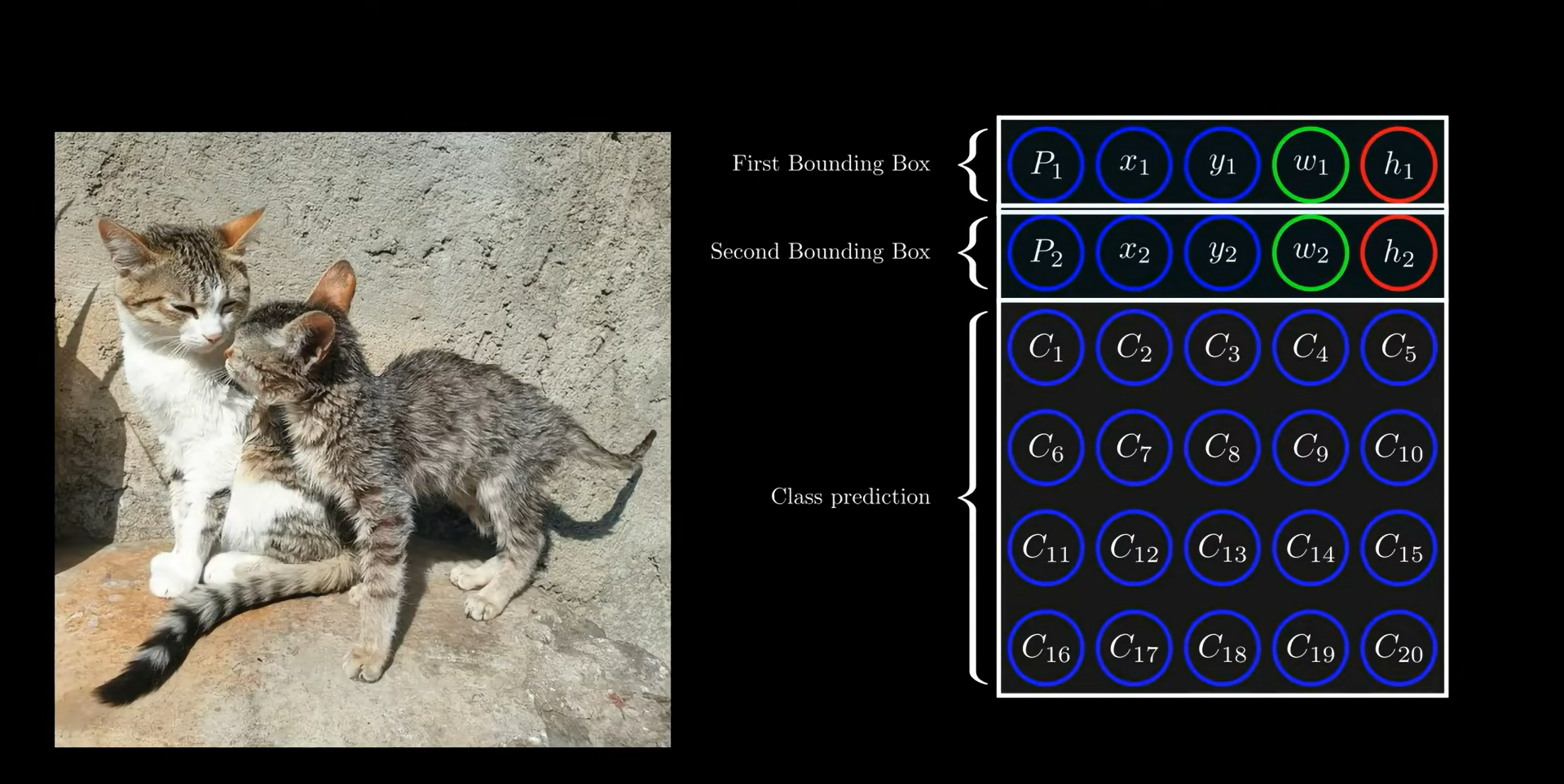
The video begins by explaining a fundamental object detection task: detecting the presence of an object (e.g., a cat) in an image and drawing a bounding box around it. The simplest method involves using a single neuron output where a value greater than 0.5 indicates the object is present, and less than 0.5 indicates absence. To draw the bounding box, four values are needed:

The X and Y coordinates of the top-left corner of the bounding box.
The width and height of the bounding box.

This allows the rectangle to be accurately drawn around the object.

Beyond just detecting the presence and location of an object, the goal extends to classifying the object type. For this purpose, 20 additional output values are introduced to classify among 20 different object categories (e.g., person, car, cat). Thus, the model is trained to predict a total of 25 values:

Output Value Index	Description
1	Object presence confidence (0 or 1)
2-3	Center X and Y coordinates of object
4-5	Width and height of bounding box
6-25	Class probabilities for 20 classes

Pasted image 20260416213918.png

Two key questions arise:

How to train a model that accurately predicts these 25 values?
How to detect multiple objects in a single image?

To detect multiple objects, the model can add five more output neurons for each additional object, allowing detection of two objects in an image. However, both objects must be from the same class, because class probabilities are shared for all bounding boxes predicted by the model.

The total number of output neurons for two objects in an image becomes 30 (2 objects × 15 neurons each). The original YOLO paper simplifies class prediction by associating only one class probability per grid cell, regardless of the number of bounding boxes predicted in that cell.

A remaining challenge is detecting more than two objects and objects belonging to different classes in the same image.

To address this, the image is divided into a $7 \times 7$ grid, where each grid cell is responsible for detecting up to two objects. This approach allows detection of up to:

7 \times 7 \times 2 = 98 objects per image

The total number of output neurons for the entire image is:

7 \times 7 \times 30 = 1470

where 30 corresponds to the output values per grid cell (2 bounding boxes × 15 values each).

A key rule: if an object appears in multiple bounding boxes, the grid cell containing the center of the object is responsible for detecting it. Other cells do not detect that object.

The video then shifts focus to the loss function, which guides training by measuring prediction error. The loss function consists of several parts:

Pasted image 20260416214111.png

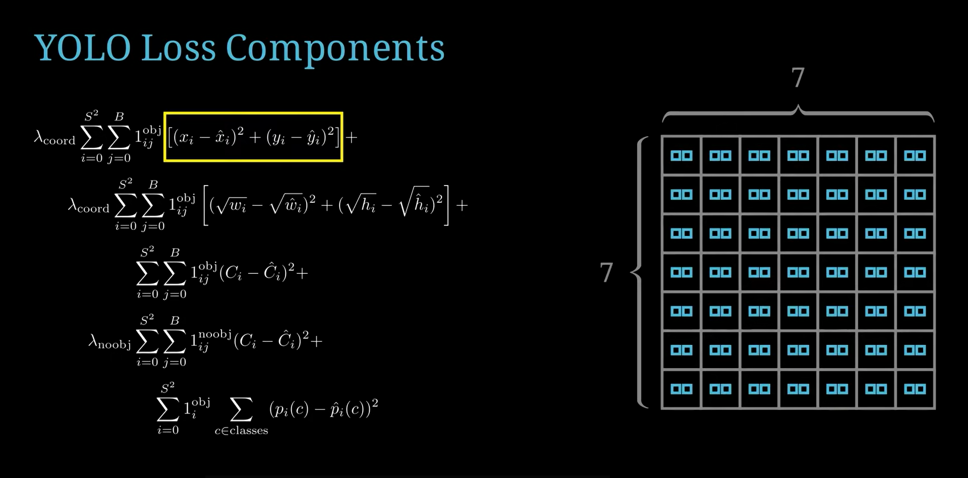
The first summation runs over all 49 grid cells ( $7 \times 7$ ).
The second summation runs over the two bounding boxes predicted per grid cell.
The loss compares actual vs. predicted coordinates of bounding box centers, widths, and heights.

Because many grid cells do not contain objects, their corresponding loss should be zero. To handle this, an indicator variable is used:

1 if the grid cell contains an object.
0 if it does not.

This "switch" ensures loss terms for empty grids do not contribute to the total loss.

The loss function includes the bounding box location loss (center coordinates) and size loss (width and height). A critical detail is the use of the square root of width and height in the loss for the size term. This is explained with an example:

Bounding Box	Ground Truth (Width × Height)	Predicted (Width × Height)	Absolute Size Error	Loss Contribution (before sqrt)	Loss Contribution (after sqrt)
Box 1	20 × 30	18 × 27	Small difference	Same as Box 2	Lower (reflects better accuracy)
Box 2	4 × 6	2 × 3	Larger relative error	Same as Box 1	Higher (focuses more on small boxes)

Pasted image 20260416214244.png

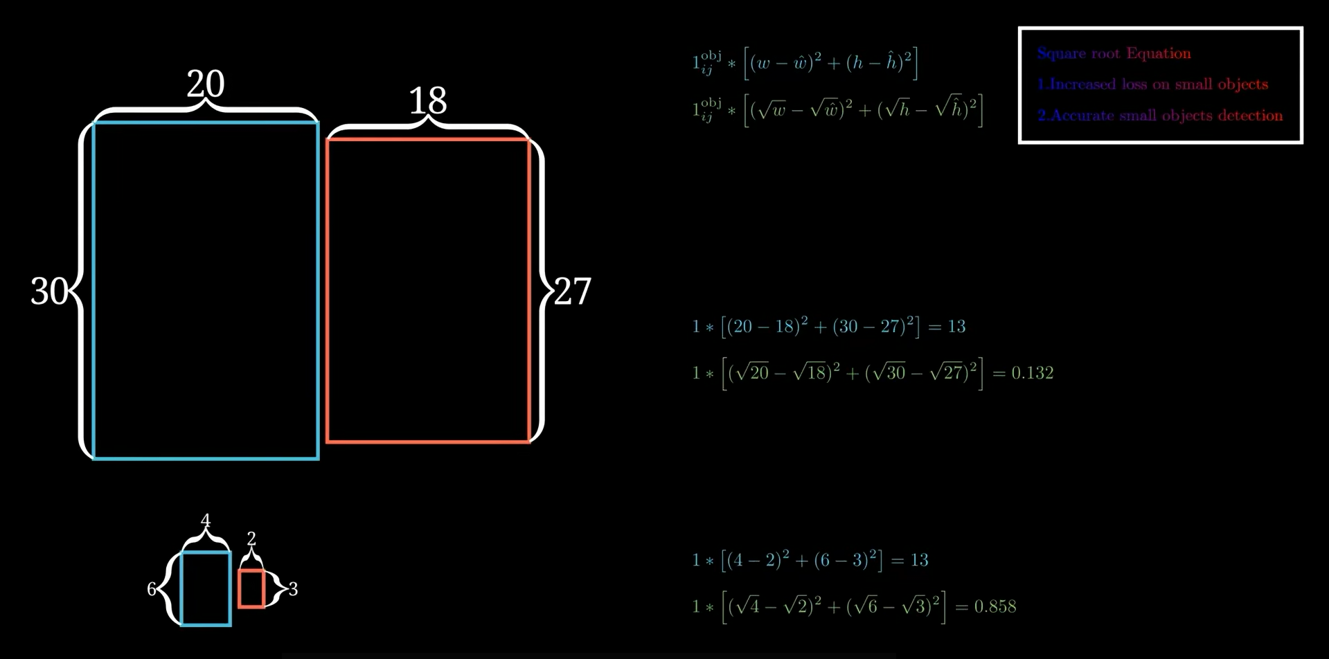
The square root transformation increases the emphasis on small bounding boxes during training, encouraging the network to predict them more accurately.

The loss also includes two parts for the confidence score of object presence:

One part corresponds to grids with objects (target = 1).
The other corresponds to grids without objects (target = 0).

To prevent the model from becoming biased towards predicting "no object" (since most grids are empty), the loss for grids without objects is weighted down by a factor of 0.5. This reduces the influence of empty grids on the training, balancing the learning process.

The final part of the loss is the class prediction loss, which compares the predicted class probabilities to the actual class for each grid cell with an object.

The loss function applies a weight of 5 to the localization losses (bounding box coordinates and sizes).
This weighting forces the model to place greater emphasis on accurate bounding box predictions.

The explanation concludes by confirming that this loss formulation corresponds to the first YOLO (You Only Look Once) paper, with the exception of one thing, the x and y coordinates in the first YOLO are for the center of the boxes, while for YOLO3 it's the top left corner.

Summary of Key Components

Component	Description
Object Detection Output	25 values per bounding box: presence (1), center (2), size (2), classes (20)
Multiple Objects Handling	Divide image into $7 \times 7$ grid; each cell predicts 2 bounding boxes with shared class probs
Total Output Neurons	$$7 \times 7 \times 30 = 1470$$
Loss Function Elements	- Localization loss (center coords, size with sqrt) - Confidence loss (object/no object) - Class prediction loss
Loss Weighting	- Object confidence loss weighted less for no-object grids (0.5) - Localization loss weighted more (5)
Key Insight	Using square root for width and height loss improves small object detection accuracy

Important Definitions and Formulas

Bounding box parameters per object:

Output vector = [\begin{matrix} p_{obj} \\ x_{center} \\ y_{center} \\ w \\ h \\ c_{1} \\ c_{2} \\ ⋮ \\ c_{20} \end{matrix}]

where $p_{obj}$ is the probability object exists, $(x_{center}, y_{center})$ is center coordinates, $w$ and $h$ are width and height, and $c_{i}$ are class probabilities.

Loss function components:

Loss = λ_{coord} \sum_{i = 0}^{48} \sum_{j = 0}^{1} 1_{i j}^{obj} [(x_{i} - {\hat{x}}_{i})^{2} + (y_{i} - {\hat{y}}_{i})^{2}] + λ_{coord} \sum_{i = 0}^{48} \sum_{j = 0}^{1} 1_{i j}^{obj} [(\sqrt{w_{i}} - \sqrt{{\hat{w}}_{i}})^{2} + (\sqrt{h_{i}} - \sqrt{{\hat{h}}_{i}})^{2}] + \dots

Where $1_{i j}^{obj} = 1$ if object exists in grid $i$ bounding box $j$ , else 0; $λ_{coord} = 5$ is a weight factor.

Concluding Remarks

The video provides a detailed walkthrough of the YOLO architecture's output design and loss function, emphasizing how bounding box coordinates, object presence, and class probabilities are predicted together.
It highlights the strategic division of the image into grid cells to handle multiple objects and the importance of the loss function's design to balance accuracy for small and large objects.
The weighting schemes in the loss prevent bias towards empty grids and encourage precise localization.
This explanation corresponds closely to the methodology described in the first YOLO paper, which revolutionized real-time object detection by framing detection as a single regression problem over spatial grids.

source: How YOLO Works

What are ResNet

ResNet, short for Residual Network, is a highly influential deep learning architecture introduced in a 2015 paper ("Deep Residual Learning for Image Recognition"). It was designed to solve a fundamental problem that occurs when trying to train extremely deep neural networks: as networks get deeper, they often start performing worse, rather than better.

Here is a detailed breakdown of how ResNet works, based on the concepts from the video:

The Problem: Losing the Signal

When building a deep neural network, you pass input data through many layers of non-linear functions (like the ReLU activation function). A major issue arises when the network becomes very deep: the original input signal gets distorted or entirely lost as it propagates through these numerous layers.

Because the network forgets the original input, the training loss can shoot upwards, meaning a deeper model might actually produce worse results than a shallower one. Essentially, you are forcing the network to do two highly difficult things simultaneously:

Retain the original input signal.
Figure out the mathematical transformation needed to turn that input into the desired output.

The Solution: Learning the "Residual"

Instead of forcing the network to learn the entire transformation from scratch, ResNet shifts the goal. It asks the network to only learn the residual—which is the difference between the input and the desired output.

The Super Resolution Analogy:

Imagine you want to turn a low-resolution image into a high-resolution image.

Standard approach: Feed the low-res image into the network and ask it to output a completely new high-res image. The network has to remember what the original image looked like while doing this.
Residual approach: Subtract the low-res image from the high-res target to find the exact difference (the missing pixels/details). You then train the network to only output that difference. Finally, you just add the original low-res input directly back onto the network's output to get your final high-res image.

By framing the problem this way, the network's job is much easier because it no longer has to focus on retaining the original input signal.

The Architecture: Residual Blocks

To apply this concept to complex tasks like image classification, ResNet architectures are built using a series of Residual Blocks (instead of standard sequential layers).

Here is the step-by-step flow inside a standard ResNet block:

Input: The data enters the block. A copy of this exact input is saved to the side (known as the "identity").
Convolution 1: The input passes through a $3 \times 3$ convolutional layer (typically with parameters that keep the dimensions exactly the same).
Batch Normalization & Activation: The features are normalized and passed through a ReLU activation function.
Convolution 2 & Batch Normalization: The data passes through a second $3 \times 3$ convolutional layer and another normalization step.
The Residual Connection (Skip Connection): At this stage, the saved "identity" (the original input to the block) is added element-wise directly onto the new features generated by the convolutions.
Final Activation: The combined data passes through a final ReLU activation function and exits the block.

Because of this skip connection, if a specific block isn't strictly necessary for the network to solve the problem, the network can easily learn to output zeros for the convolutional layers. The block will then simply output the "identity function" (the exact original input), taking no penalty to the loss function. This mechanism is what allows ResNets to be incredibly deep without destabilizing.

Handling Dimension Mismatches

For the element-wise addition in step 5 to work, the dimensions of the saved input and the new feature map must be identical. However, in tasks like image classification, neural networks need to periodically downsample the image dimensions (reduce height and width) while increasing the number of feature channels.

When a ResNet block needs to downsample, it changes the stride of its first convolution to 2. This halves the height and width and doubles the channels. Now, the saved "identity" input no longer matches the dimensions of the new features.

To fix this dimension mismatch, the input identity must also be adjusted before it is added. There are two solutions:

Zero Padding: Pad the extra channel dimensions with zeros and use a stride of 2 to skip pixels. This introduces no new parameters, but wastes computation on meaningless zero values.
$1 \times 1$ Convolution (Preferred): Pass the identity input through a $1 \times 1$ convolutional layer with a stride of 2, and double the number of convolutional filters. This correctly halves the spatial dimensions and doubles the channels to perfectly match the main network features, ensuring only real, meaningful information is added.

How Residual Blocks Work

To understand how a Residual Block forces a network to learn the "difference" (the residual) and why those skip connections are so crucial, we need to look at the math and the flow of information during training.

Here is exactly how the architecture enforces this concept.

1. How the Block Forces the Network to Learn the "Difference"

Imagine a specific point in the middle of a neural network. You have an input coming into a block of layers, let's call it $x$ . You also have an ideal, perfect output that you want this block to produce so the network can accurately classify the image. Let's call that ideal output $H (x)$ .

In a standard, non-residual network, the convolutional layers within that block are tasked with learning the entire transformation. Their weights must figure out how to take $x$ and manipulate it directly into $H (x)$ .

In a Residual Block, the architecture physically changes the equation.

Instead of sending $x$ just through the convolutional layers, the block takes a copy of $x$ and routes it around the layers, adding it directly to the output at the very end.

Because the final output of the block is now mathematically forced to be whatever the layers produced plus the original input $x$ , the layers inside the block can no longer output $H (x)$ . If they did, the final output would be $H (x) + x$ , which is incorrect.

To ensure the final output is the ideal $H (x)$ , the convolutional layers are mathematically forced to learn a new function, let's call it $F (x)$ , where:

$F (x) = H (x) - x$

$F (x)$ is the residual—the exact mathematical difference between the input you have and the output you want.

Analogy: If you are at mile marker 5 ( $x$ ) and you need to be at mile marker 12 ( $H (x)$ ), a standard network tries to learn the number "12". A residual network simply passes the "5" forward, and forces the layers to learn the operation "+7".

2. Why Add the Original Input? (The Power of the Skip Connection)

The routing of the input $x$ around the layers is called a skip connection or shortcut connection. Adding this original input back into the stream solves the two biggest problems in deep learning:

A. Providing an "Identity" Default (Doing No Harm)

In very deep networks, not every layer is necessary. Sometimes, adding more layers makes the model worse because those extra layers distort a perfectly good signal.

If a standard network decides a layer is unnecessary, it is incredibly difficult for it to learn how to pass the data through completely unchanged (known as the identity function) because the data has to pass through complex matrix multiplications and non-linear activation functions (like ReLU).

With a skip connection, if the network decides a block is unnecessary, it has a trivially easy solution: it just pushes the weights of the convolutional layers to zero.

If the layers output $0$ , then the block's final equation becomes:

$0 + x = x$ .

The input passes through perfectly unchanged. This guarantees that adding more layers to a ResNet will never degrade its performance; at worst, the extra layers will just do nothing.

B. The Gradient Superhighway (Stopping Vanishing Gradients)

During training, neural networks learn by calculating the "error" at the final output and passing that error backward through every single layer to update the weights (a process called backpropagation).

In standard networks, as this error signal passes backward through dozens or hundreds of layers, it gets multiplied repeatedly. If the numbers are small, the error signal quickly shrinks to near zero—meaning the early layers never receive a strong enough signal to learn anything. This is the vanishing gradient problem.

Skip connections act as an unobstructed superhighway for these error signals. Because the addition operation ( $F (x) + x$ ) simply distributes the gradient equally when flowing backward, the error signal can bypass the complex convolutional layers and flow directly back to the earlier parts of the network at full strength. This is what allows ResNets to be hundreds, or even thousands, of layers deep without the training process collapsing.

To understand these two mechanisms, we have to look closely at the underlying mathematics of how neural networks learn: the Loss Function and the Chain Rule of Calculus.

Networks do not make conscious "decisions," nor do they know in advance which layers are useful. Everything is driven by the mathematical optimization process called Gradient Descent.

Here is the exact breakdown of how the network learns to ignore useless blocks and how the skip connection guarantees the gradient survives.

1. How a Network "Decides" a Block is Unnecessary

During training, the network's singular goal is to minimize the Loss (the error between its prediction and the true target). It does this by updating the weights of its convolutional layers.

Imagine a specific Residual Block where the optimal mathematical move for the network is actually to do nothing—the input $x$ is already perfect, and passing it through more convolutional layers will only distort it and increase the Loss.

Here is how the optimization process naturally "turns off" that block:

The Error Signal: Because the extra convolution increased the Loss, the backpropagation algorithm sends a strong error signal back to that specific block.
Weight Decay & Gradient Update: The gradient descent equation tells the weights ( $W$ ) inside the block to adjust themselves in the opposite direction of the error. Repeatedly, the math pushes these specific weights closer and closer to zero to stop them from making the prediction worse.
The ResNet Advantage: As the weights $W$ approach zero, the output of the convolutional layers, $F (x)$ , also approaches zero.

Because the block's final equation is $y = F (x) + x$ , as $F (x) \to 0$ , the block naturally becomes $y = 0 + x = x$ . The block seamlessly transforms into the identity function.

Why standard networks fail here: If a standard, non-residual network tries this exact same mathematical optimization, pushing its weights to zero results in $y = 0$ . The block effectively deletes the entire image/signal, causing the network's performance to collapse. The addition operation in ResNet is what makes zeroing-out safe.

2. How the Addition Node Distributes the Gradient (The Chain Rule)

The true magic of the skip connection happens during backpropagation. To understand how the gradient is distributed equally, we apply the Chain Rule of calculus to the Residual Block's addition node.

Let:

$x$ be the input to the block.
$F (x)$ be the output of the convolutional layers.
$y = F (x) + x$ be the final output of the block.
$L$ be the final Loss of the entire network.

During backpropagation, the block receives the gradient of the loss from the layers ahead of it: $\frac{\partial L}{\partial y}$ .

The block's job is to pass this gradient backward to the layers before it, which means calculating $\frac{\partial L}{\partial x}$ .

According to the Chain Rule:

\frac{\partial L}{\partial x} = \frac{\partial L}{\partial y} \cdot \frac{\partial y}{\partial x}

Now, let's find the derivative of the block's operation, $\frac{\partial y}{\partial x}$ :

y = F (x) + x

\frac{\partial y}{\partial x} = \frac{\partial F (x)}{\partial x} + \frac{\partial x}{\partial x}

\frac{\partial y}{\partial x} = F^{'} (x) + 1

Now, substitute this back into our Chain Rule equation:

\frac{\partial L}{\partial x} = \frac{\partial L}{\partial y} \cdot (F^{'} (x) + 1)

\frac{\partial L}{\partial x} = (\frac{\partial L}{\partial y} \cdot F^{'} (x)) + \frac{\partial L}{\partial y}

The meaning of this final equation:

Look at the two terms on the right side of the plus sign. This shows exactly how the addition node mathematically splits the backward-flowing gradient into two separate paths:

$\frac{\partial L}{\partial y} \cdot F^{'} (x)$ (The Convolution Path): This is the gradient flowing backward through the complex convolutional layers. Because $F^{'} (x)$ involves the weights of those layers, this number can easily become incredibly tiny (vanishing gradient) or massive (exploding gradient).
$\frac{\partial L}{\partial y}$ (The Skip Connection Path): Notice there is no multiplier here (because the derivative of $x$ is 1). This is the exact, pure, original gradient arriving from the future layers, completely untouched.

The Conclusion:

Because these two paths are added together, it does not matter if the convolution path completely dies and becomes $0$ . The equation simply becomes:

\frac{\partial L}{\partial x} = 0 + \frac{\partial L}{\partial y}

The pure gradient ( $\frac{\partial L}{\partial y}$ ) is guaranteed to survive and pass directly to the previous layers. The "+ 1" from the calculus derivative is the mathematical engine that creates the unobstructed gradient superhighway.

Sources: Gemini and ResNet (actually) explained in under 10 minutes

Transfer Learning Example (VGG16)