Lecture 6 - CNN Cont

1. Data Pre-processing

Before you even touch a CNN, your data needs to be prepped. Raw data is messy, and neural networks perform best when the input data is uniform.

The lecture highlights four key preprocessing techniques to improve performance and prevent overfitting:

Normalization: The goal is to shift your input variables so they roughly follow a standard Gaussian distribution $N (0, 1)$ . To do this, you compute the mean ( $μ$ ) and standard deviation ( $σ$ ) from your training set. You subtract the mean from the training samples and divide the result by the standard deviation: $\frac{x - μ}{σ}$ .
Data Augmentation: If you don't have enough data, you can artificially create more by altering existing images. Common techniques include flipping, random cropping, adjusting contrast, and adding tint.
Early Stopping: This is a technique to stop the model before it memorizes the training data (overfits). You monitor the error on a separate validation set. As training progresses, the training error will decrease, but eventually, the validation error will start to increase. You stop the training exactly when that validation error begins to rise.
Dropout: To prevent neurons from becoming overly dependent on each other, Dropout randomly "turns off" certain nodes during each training epoch. This means the network effectively acts as a different architecture at every training epoch, which creates a robust effect very similar to training an ensemble of models.

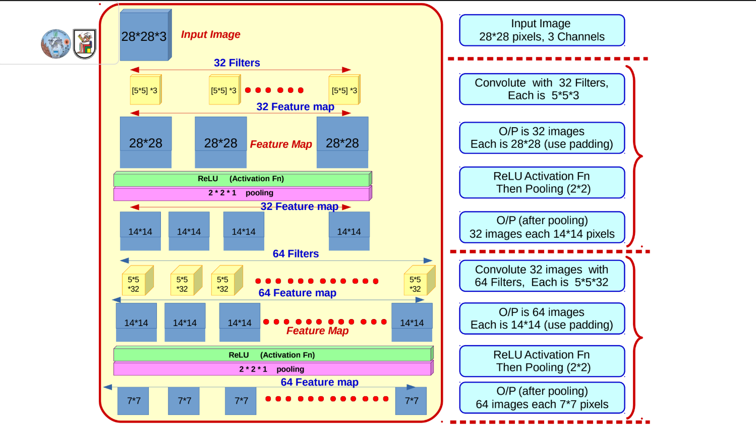
2. CNN Architecture and Feature Maps

The slides walk through a highly specific architectural example to show exactly how images are transformed from raw pixels into flattened feature vectors.

Let's trace the math of how an image moves through this network:

The Input: You start with an image that is $28 \times 28$ pixels with 3 color channels ( $28 \times 28 \times 3$ ).
First Convolution: You apply 32 different filters, each sized $5 \times 5 \times 3$ . Using padding, the spatial dimensions remain the same, resulting in 32 feature maps of size $28 \times 28$ .
Activation & Pooling: You pass the output through a ReLU activation function, then apply a $2 \times 2$ Max Pooling layer. Pooling halves the dimensions, leaving you with 32 feature maps of size $14 \times 14$ .
Second Convolution: You take those 32 maps and apply 64 new filters. Because the previous depth was 32, these filters must have a matching depth of 32 (sized $5 \times 5 \times 32$ ). This results in 64 feature maps of size $14 \times 14$ .
Second Activation & Pooling: After another ReLU and $2 \times 2$ Max Pooling step, the spatial dimensions halve again, resulting in 64 feature maps of size $7 \times 7$ .
Flattening: The 3D tensor ( $7 \times 7 \times 64$ ) is flattened into a single 1D vector containing 3,136 values ( $7 \times 7 \times 64 = 3136$ ).
Fully Connected Layers: This vector is fed into a hidden layer of 1,024 neurons, and finally into an output layer of 10 neurons (representing 10 possible classes).

Pasted image 20260331222837.png

Pasted image 20260331222857.png

3. Weight Updating & The Softmax Function

At the very end of the network, those final 10 neurons use the Softmax Activation function to convert raw mathematical scores into clean, readable probabilities that sum to 1.

The Softmax formula is:

σ (z)_{i} = \frac{e^{z_{i}}}{\sum_{j = 1}^{K} e^{z_{j}}}

Here, $e^{z_{i}}$ is the exponential of the target class score, and it is divided by the sum of the exponentials of all $K$ class scores to generate the final probability (e.g., $P (class B) = 0.95$ ).

Once the prediction is made, the network calculates the Cross-Entropy loss by comparing the prediction against the True One-Hot Labels, and uses backpropagation to update the weights across all the layers.

4. Tracking Spatial Dimensions (The Math)

The lecture includes a slide breaking down the famous AlexNet architecture, which reveals the exact formula for how spatial dimensions shrink during convolutions and pooling.

If you have an input size ( $W$ ), a filter size ( $F$ ), padding ( $P$ ), and a stride ( $S$ ), the output dimension is calculated as:

Output Size = \frac{W - F + 2 P}{S} + 1

Example from the slides:

You start with a $227 \times 227$ image.
You apply a $11 \times 11$ Convolution filter with a stride of 4.
Math: $(227 - 11) / 4 + 1 = 54 + 1 = 55$ .
The new spatial dimension is $55 \times 55$ .
Next, you apply a $3 \times 3$ Max Pool with a stride of 2.
Math: $(55 - 3) / 2 + 1 = 26 + 1 = 27$ .
The new spatial dimension is $27 \times 27$ .

4.2. Num of Parameters

Pasted image 20260331223319.png

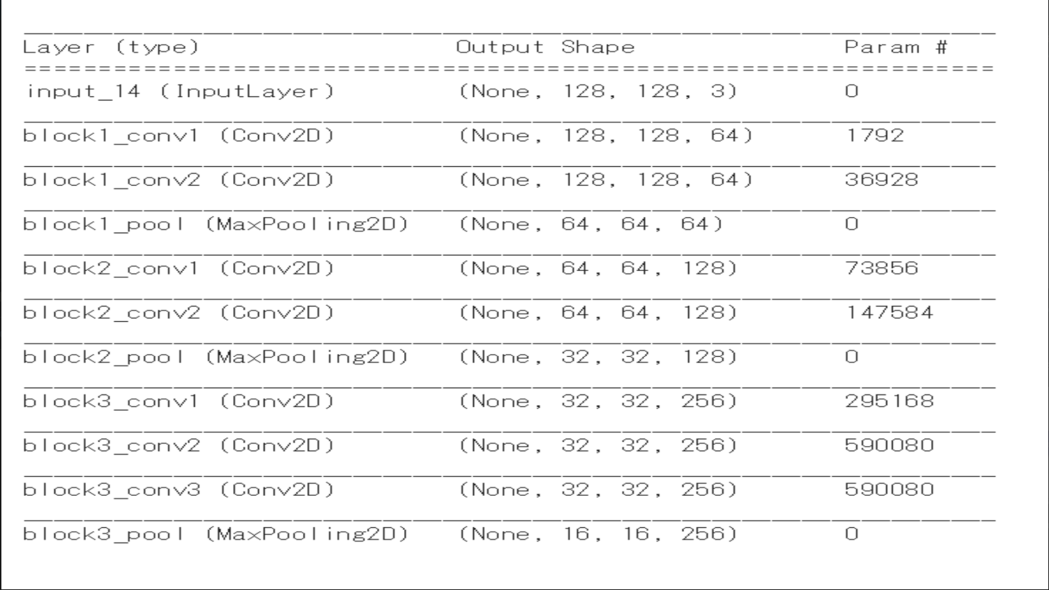
To compute the number of parameters in a Convolutional (Conv2D) layer, you need to know the dimensions of the filter (kernel) being used, the depth (number of channels) of the input, and the number of filters applied in the current layer.

The general formula is:

P a r a m e t e r s = (F_{w} \times F_{h} \times D_{i n} + 1) \times K

Where:

$F_{w} \times F_{h}$ : The width and height of the filter (kernel).
$D_{i n}$ : The depth of the input volume (number of channels from the previous layer).
$1$ : The bias term (each filter has one bias weight).
$K$ : The number of filters in the current layer.

We'll assume 3x3 filter size

Here is the step-by-step mathematical breakdown for the first four Conv2D layers based on lecture example:

1. `block1_conv1`

Input Depth: 3 (from the input_14 layer shape 128, 128, 3)
Filter Size: 3x3
Number of Filters: 64 (from the output shape 128, 128, 64)
Weights per filter: 3 * 3 * 3 = 27 weights
Bias per filter: 1
Calculation: (27 + 1) * 64 = 1792 parameters

2. `block1_conv2`

Input Depth: 64 (from the previous block1_conv1 output)
Filter Size: 3x3
Number of Filters: 64 (from the output shape 128, 128, 64)
Weights per filter: 3 * 3 * 64 = 576 weights
Bias per filter: 1
Calculation: (576 + 1) * 64 = 36928 parameters

(Note: The block1_pool layer has 0 parameters because pooling layers only perform a fixed mathematical operation like taking the maximum value; they do not have learnable weights).

3. `block2_conv1`

Input Depth: 64 (from the previous block1_pool output)
Filter Size: 3x3
Number of Filters: 128 (from the output shape 64, 64, 128)
Weights per filter: 3 * 3 * 64 = 576 weights
Bias per filter: 1
Calculation: (576 + 1) * 128 = 73856 parameters

4. `block2_conv2`

Input Depth: 128 (from the previous block2_conv1 output)
Filter Size: 3x3
Number of Filters: 128 (from the output shape 64, 64, 128)
Weights per filter: 3 * 3 * 128 = 1152 weights
Bias per filter: 1
Calculation: (1152 + 1) * 128 = 147584 parameters

5. Transfer Learning (TBC) Not in Mid

Finally, the lecture formally touches on Transfer Learning. Rather than building and training massive architectures like the one above from scratch—which requires enormous amounts of data and compute—you take an existing Model (Model 01) that was already trained on a massive dataset (Data 01).

You then transfer that pre-learned knowledge (the weights and feature-extracting capabilities) to a new, structurally similar Model (Model 02) to make predictions on a new, smaller dataset (Data 02).