1. The Core Concept: Uninformed (Blind) Search

Search algorithms operate over models of the world to find a path or configuration that satisfies a goal. Uninformed search (also called blind search) strategies only use the information available in the problem definition itself. They evaluate path costs but possess no heuristic information about how far a given state is from the actual goal.

Because they explore without a "sense of direction," they can often be inefficient for exceptionally large search spaces.

2. Breadth-First Search (BFS)

BFS explores the search space tier by tier.

• Strategy: It always expands the shallowest unexpanded node first.
  
  
• Implementation: The fringe (the collection of nodes waiting to be expanded) is managed as a FIFO (First-In, First-Out) queue.
  
  
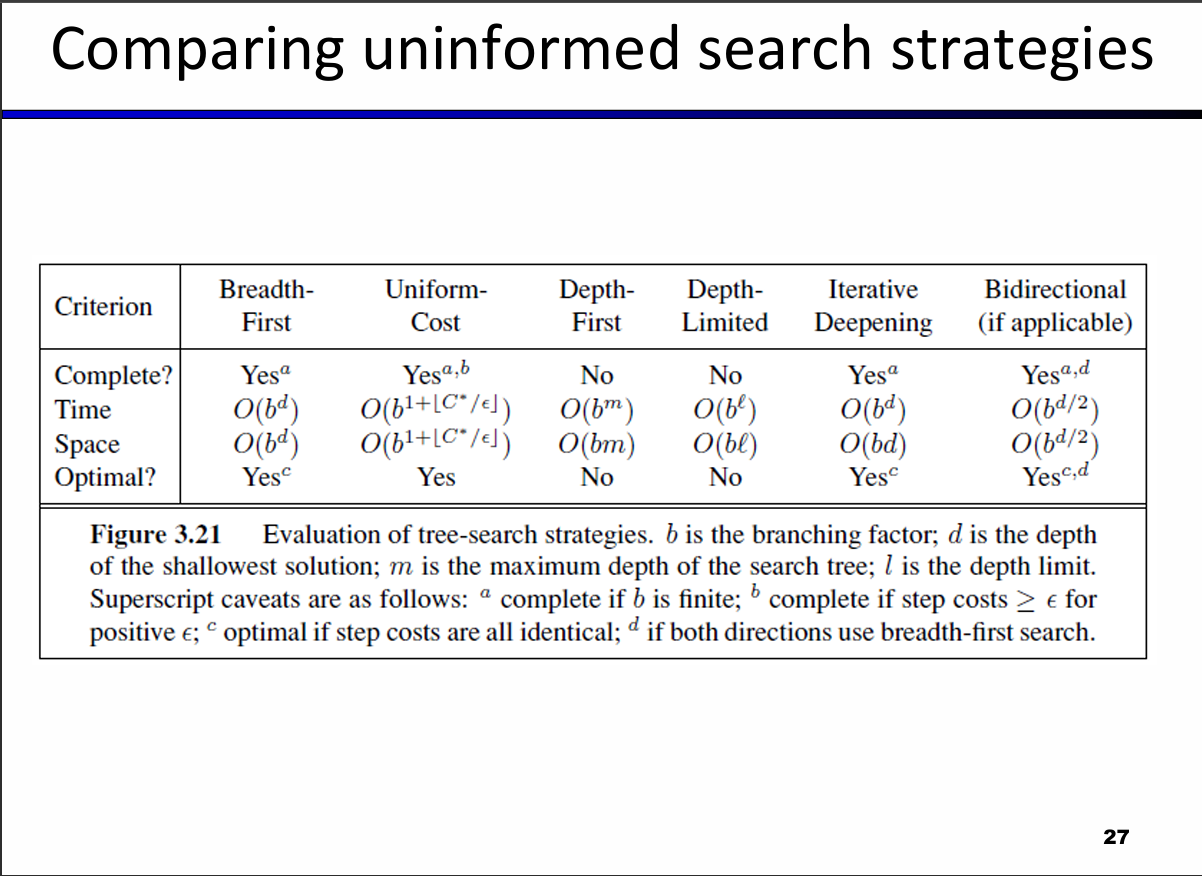
• Complexity: Both time and space complexities are $O(b^d)$, where $b$ is the branching factor and $d$ is the depth of the goal. Space is a significant bottleneck because BFS must keep roughly the entire last tier of nodes in memory.
  
  
• Properties:
  • Complete: Yes, it is guaranteed to find a solution if the branching factor is finite.
    
    
  • Optimal: Yes, but only if every step costs exactly 1.

Example with Code "Cannibals and Missionaries Problem"

def breadth_first_search(start_state, goal_state):

    # Fringe managed as a FIFO queue: stores tuples of (current_state,                   path_history)
    fringe = [(start_state, [])]

    # Visited set prevents infinite loops and redundant exploration
    explored = set([start_state])

    nodes_expanded = 0

    while fringe:

        # Pop from the shallowest end of the queue
        current_state, path = fringe.pop(0)

        # Goal test
        if current_state == goal_state:
            print(f"Goal found! Nodes expanded: {nodes_expanded}")
            return path + [(current_state, "Goal Reached")]

        nodes_expanded += 1

        # Expand node
        for next_state, action in get_successors(current_state):

            if next_state not in explored:
                explored.add(next_state)
                # Append to the back of the queue (FIFO)
                fringe.append((next_state, path + [(current_state, action)]))
    return None

3. Depth-First Search (DFS)

DFS dives as deep as possible down a single path before backtracking.

• Strategy: It expands the deepest unexpanded node first.
  
  
• Implementation: The fringe is managed as a LIFO (Last-In, First-Out) stack.
  
  
• Complexity: The time complexity is $O(b^m)$, where $m$ is the maximum depth of the search tree. However, its primary advantage is its space complexity, which is only $O(bm)$.
  
  
• The Space Advantage: DFS only needs to store a single path from the root to a leaf node, alongside the unexpanded sibling nodes on that path. Once a node is fully explored, it is removed from memory.
  
  
• Properties:
  
  
  • Complete: No. It can fail in infinite-depth spaces or get trapped in cycles.
    
    
  • Optimal: No. It will simply return the "leftmost" solution it encounters, regardless of whether a shallower or cheaper solution exists.

The choice between Breadth-First Search (BFS) and Depth-First Search (DFS) often comes down to the shape of the search space (how wide vs. how deep it is) and what you know about the location of the goal.

When BFS Outperforms DFS

BFS explores the search space level by level, radiating outward from the start node. It is generally the better choice in these scenarios:

1. The goal is shallow (close to the root): Because BFS checks every node at depth 1, then depth 2, and so on, it will quickly find a solution that requires only a few steps without wasting time exploring deeply unrelated paths.

2. You need the shortest path: In an unweighted graph, the first time BFS reaches a goal, it is mathematically guaranteed to be the shortest path (fewest number of edges). DFS, by contrast, might plunge down a long, winding path and return a highly suboptimal solution just because it found it first.

3. The search tree is infinite or extremely deep: If the state space has paths that go on forever (or are deep enough to cause a stack overflow), DFS can easily get trapped exploring a useless, bottomless branch. BFS is complete, meaning it is guaranteed to find a solution if one exists, regardless of infinite depths elsewhere in the tree.

When DFS Outperforms BFS

DFS plunges as deeply as possible down a single path before backtracking. Its primary advantage is memory conservation. It is the better choice in these scenarios:

1. Memory is strictly limited: This is the most common reason to choose DFS. BFS must store every node of the current depth level in memory (its fringe). In a tree with a high branching factor, the space required by BFS grows exponentially ($O(b^d)$). DFS only needs to store the single path from the root to the current node, plus the unexpanded sibling nodes along that path, making its memory footprint linear ($O(bm)$).

2. The goal is known to be deep: If you know the solution requires many steps (e.g., solving a maze, where the exit is at the far end), DFS will dive straight toward the bottom of the tree and may stumble upon the goal much faster than BFS, which would waste time exhaustively checking every single shallow dead-end first.

3. You need to visit every node anyway: For tasks like cycle detection, topological sorting, or counting the total number of connected components in a graph, you must traverse the entire structure. Since neither algorithm can stop early, the massive memory efficiency of DFS makes it the superior choice.

4. Iterative Deepening

This strategy attempts to combine the best properties of both BFS and DFS.

• Strategy: It runs a standard DFS, but artificially limits the depth. If no solution is found at depth limit 1, it runs DFS again with depth limit 2, then 3, and so on.
  
  
• Why it works: While it seems wastefully redundant to keep restarting the search, the vast majority of nodes in a tree exist at the lowest level. Therefore, the overhead of repeating the upper levels is relatively negligible. You gain the $O(bm)$ space advantage of DFS alongside the completeness and shallow-solution advantages of BFS.

5. Uniform-Cost Search (UCS)

Standard BFS evaluates the number of steps, but UCS evaluates the actual cost of the path.

• Strategy: It expands the cheapest node first based on the cumulative cost from the start node. It essentially explores the space in "increasing cost contours".
  
  
• Implementation: The fringe is managed as a priority queue, where the priority is determined by the cumulative path cost.
  
  
• Complexity: Time and space complexities are bounded by $O(b^{1+\lfloor C^{\ast }/ϵ\rfloor })$, where $C^{\ast }$ is the cost of the optimal solution and $ϵ$ is the minimum step cost.
  
  
• Properties:
  
  
  • Complete: Yes, assuming the best solution has a finite cost and the minimum step cost is strictly positive.
    
    
  • Optimal: Yes, it is guaranteed to find the least-cost path.
    
    
  • Drawback: It explores options in every possible "direction" blindly because it has no information about where the goal is actually located.