Lecture 8 - Image Restoration and Reconstruction

1. Image Restoration vs. Image Enhancement

First, it is crucial to understand the difference between these two concepts:

Image Enhancement is subjective; it manipulates an image to make it look more pleasing to the human visual system (like bumping up the contrast on a dark photo).
Image Restoration is objective; it assumes the image was originally high-quality but was mathematically degraded by a specific process (like motion blur, camera misfocus, or sensor noise). The goal is to model that exact degradation and mathematically "undo" it to recover the original image.

2. Understanding Noise Models

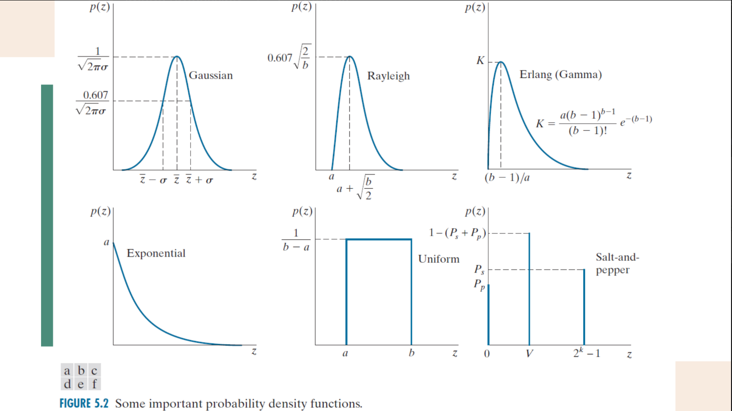
Noise in digital images usually occurs during acquisition (due to sensor temperature or lighting) or transmission (due to electrical interference). Because noise is a random fluctuation in pixel values, it is mathematically modeled using probability density functions (PDFs). Common models include Gaussian (the most common), Rayleigh, Erlang, Exponential, Uniform, and Impulse (Salt-and-Pepper) noise.

What is an Image Noise Model?

In digital image processing, noise is defined as a random fluctuation in pixel values. Because these fluctuations are random, we mathematically characterize them using Probability Density Functions (PDFs). A PDF is an equation that links a specific pixel intensity value ( $z$ ) with its mathematical probability of occurring.

Here is a detailed breakdown of the six primary noise models discussed:

1. Gaussian Noise (The Most Common)

Gaussian noise is the most frequently used model because it closely approximates noise that occurs in real-world situations, such as sensor noise during image acquisition.

PDF Shape: A symmetrical, bell-shaped curve.
Key Characteristics: The distribution is centered around a mean value ( $\bar{z}$ ). There is a 68% probability that a noise pixel's value falls within one standard deviation ( $\bar{z} \pm σ$ ), and a 95% probability it falls within two standard deviations ( $\bar{z} \pm 2 σ$ ).
Mathematical Formula:
$p (z) = \frac{1}{\sqrt{2 π} σ} e^{\frac{- (z - \bar{z})^{2}}{2 σ^{2}}}$

2. Impulse Noise (Salt-and-Pepper)

Unlike Gaussian noise which alters pixels by a random continuous amount, impulse noise completely replaces a pixel's value with either maximum brightness or maximum darkness. It typically arises from quick transients, like faulty switching during imaging.

PDF Shape: Two distinct, isolated vertical spikes (impulses) at the extreme ends of the intensity scale.
Key Characteristics: It creates distinct black and white dots over the image.
- Salt: Maximum intensity (white), located at $z = 2^{k} - 1$ with a probability of $P_{s}$ .
- Pepper: Minimum intensity (black), located at $z = 0$ with a probability of $P_{p}$ .
Mathematical Formula:
$p (z) = {\begin{cases} P_{s} & for z = 2^{k} - 1 \\ P_{p} & for z = 0 \\ 1 - (P_{s} + P_{p}) & for z = V \end{cases}$
(Where $V$ represents the uncorrupted image pixels).

3. Uniform Noise

PDF Shape: A perfectly flat, rectangular block.
Key Characteristics: The noise values are evenly distributed across a specific range from $a$ to $b$ . Every pixel intensity within this range has the exact same probability of occurring.

4. Rayleigh Noise

PDF Shape: An asymmetrical curve that is skewed heavily to the right.
Key Characteristics: The probability is exactly zero for any value below a certain threshold ( $a$ ). Once it hits $a$ , it spikes rapidly and then features a long, tapering tail to the right.

5. Erlang (Gamma) Noise

PDF Shape: Similar to the Rayleigh distribution, it is an asymmetrical curve skewed to the right.
Key Characteristics: It is often used to model noise in laser imaging or synthetic aperture radar. While it looks visually similar to Rayleigh noise, it is governed by a different mathematical base (utilizing factorials and a slightly different curve decay).

6. Exponential Noise

PDF Shape: A curve that starts at a maximum probability at a threshold ( $a$ ) and exponentially decays as the intensity value increases.
Key Characteristics: It is a special case of the Erlang distribution and is often used in modeling noise in laser imaging systems.

Summary Comparison Table

Noise Model	Visual Shape of PDF	Primary Visual Effect on an Image
Gaussian	Symmetrical Bell Curve	Adds a general, uniform "grain" across the entire image.
Salt-and-Pepper	Two extreme spikes	Adds isolated, highly visible white (salt) and black (pepper) dots.
Uniform	Flat Rectangle	Washes out the image with a completely even distribution of noise.
Rayleigh	Right-skewed curve	Adds noise that heavily favors mid-to-high intensity values.
Erlang (Gamma)	Right-skewed curve	Similar visual degradation to Rayleigh, but mathematically distinct.
Exponential	Decaying slope	Noise heavily concentrated at a specific low value, fading out at higher intensities.

Pasted image 20260402011441.png

example on how to apply noise models here

Comparison 1: Spatial Domain Filters (For Random Noise)

When an image is degraded only by random additive noise, we use Spatial Filters, which operate directly on the pixels. They are divided into three main families:

A. Mean Filters (Averaging)

These filters calculate a specific mathematical average of the pixels within a neighborhood window.

Filter Type	How it Works	Best Used For	Drawbacks	Mathematical Equation
Arithmetic Mean	Computes the standard average of pixels in the window.	General smoothing and reducing general noise.	Blurs the image and loses sharp details.	$\hat{f} (x, y) = \frac{1}{m n} \sum_{(s, t) \in S_{x y}} g (s, t)$
Geometric Mean	Multiplies pixels together, then takes the $m n$ -th root.	General smoothing.	Performs similarly to arithmetic mean but retains slightly more detail.	$\hat{f} (x, y) = {[\prod_{(s, t) \in S_{x y}} g (s, t)]}^{\frac{1}{m n}}$
Harmonic Mean	Divides the total number of pixels by the sum of their reciprocals.	Works well for Gaussian noise and "salt" noise (white pixels).	Fails completely for "pepper" noise (black pixels).	$\hat{f} (x, y) = \frac{m n}{\sum_{(s, t) \in S_{x y}} \frac{1}{g (s, t)}}$
Contraharmonic Mean	Uses a fractional formula controlled by an order parameter, $Q$ .	Excellent for Salt-and-Pepper noise. Use $Q > 0$ to eliminate pepper noise, or $Q < 0$ to eliminate salt noise (Q = 0, -1 maps to Arithmetic and Harmonic respectively).	Choosing the wrong sign for $Q$ drastically worsens the image.	$\hat{f} (x, y) = \frac{\sum_{(s, t) \in S_{x y}} g (s, t)^{Q + 1}}{\sum_{(s, t) \in S_{x y}} g (s, t)^{Q}}$

B. Order Statistics Filters (Sorting)

Instead of doing math on the pixel values, these filters sort the neighborhood pixels from lowest to highest and pick a specific one.

Filter Type	How it Works	Best Used For
Median	Sorts pixels and selects the exact middle value.	Extremely effective for Salt-and-Pepper (impulse) noise. It removes extreme values without blurring edges as much as linear filters.
Max	Sorts pixels and selects the highest value.	Finding the brightest points in an image; effectively reduces "pepper" (black) noise.
Min	Sorts pixels and selects the lowest value.	Finding the darkest points in an image; effectively reduces "salt" (white) noise.
Midpoint	Averages only the absolute highest (Max) and lowest (Min) values.	Works best for randomly distributed Gaussian or Uniform noise.
Alpha-Trimmed Mean	Deletes the $d / 2$ lowest and $d / 2$ highest values, then averages the remaining pixels. When 𝑑 = 0, the alpha-trimmed filter reduces to the arithmetic mean filter. If 𝑑 = 𝑚𝑛 −1, the filter becomes a median filter.	Great for situations with multiple types of noise mixed together (e.g., Salt-and-Pepper mixed with Gaussian).

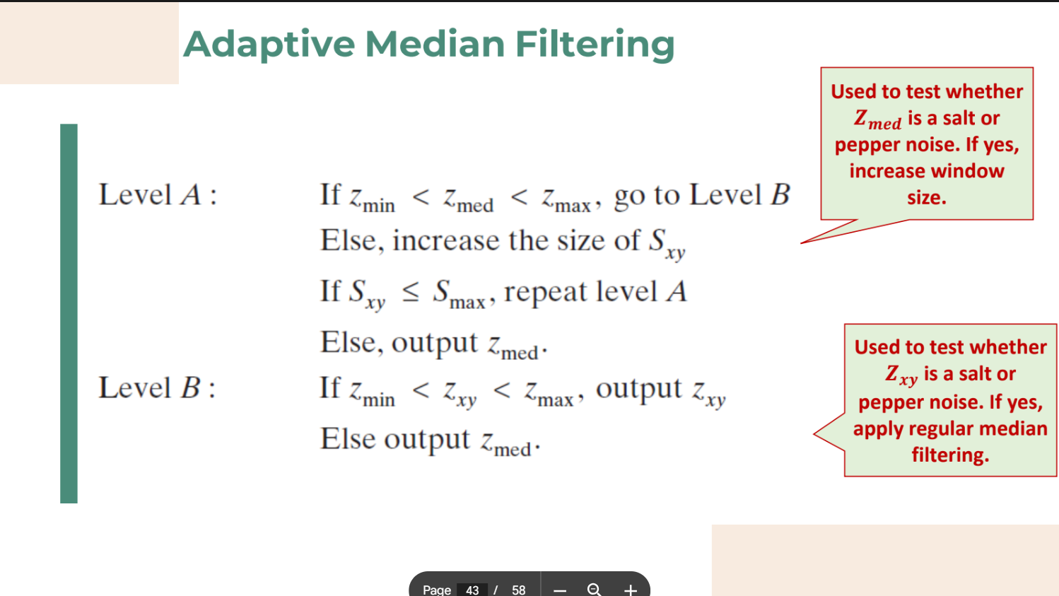
C. Adaptive Filters

Unlike the filters above which blindly apply the exact same rule to every pixel, Adaptive Filters (like the Adaptive Median Filter) change their behavior based on the local image characteristics.

How it works: It looks at a pixel neighborhood. If it detects a high density of impulse noise, it automatically increases its window size to find a clean median value. If it detects a clean pixel, it leaves it alone.
Result: It can handle heavily dense salt-and-pepper noise while preserving much sharper details than a standard median filter.

Pasted image 20260402013452.png

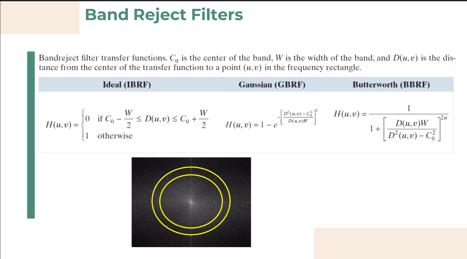
Comparison 2: Frequency Domain Filters (For Periodic Noise)

While Spatial Filters are great for random noise, Frequency Domain Filters are required for Periodic Noise. This noise usually comes from electromagnetic interference and appears as repeating, uniform patterns over the image (which look like concentrated bursts of energy in a Fourier transform).

Filter Type	Function	Use Case
Band Reject	Removes a specific "ring" or band of frequencies ( $D_{1}$ to $D_{h}$ ) while leaving lower and higher frequencies intact.	Highly effective at removing broad periodic noise patterns.
Band Pass	The exact opposite of Band Reject. It only allows a specific band of frequencies to pass through.	Used to isolate a specific frequency range for analysis. $H_{b p} (u, v) = 1 - H_{b r} (u, v)$ .
Notch Reject	Instead of removing a whole ring, it removes highly specific, pinpoint frequency components (appearing in symmetric pairs around the origin).	Perfect for removing a clearly defined interference pattern caused by an electrical disturbance (like the interference grid in a satellite photo).

Pasted image 20260402013721.png