Lecture 7 - Filtering in the Frequency Domain - Ch4

The Frequency Domain Filtering Process

This lecture builds on the basics of the Fourier Transform to show how we practically apply filters to images. Because spatial convolution is equivalent to frequency domain multiplication, we can process images much faster by multiplying their frequency components by a filter function $H (u, v)$ .

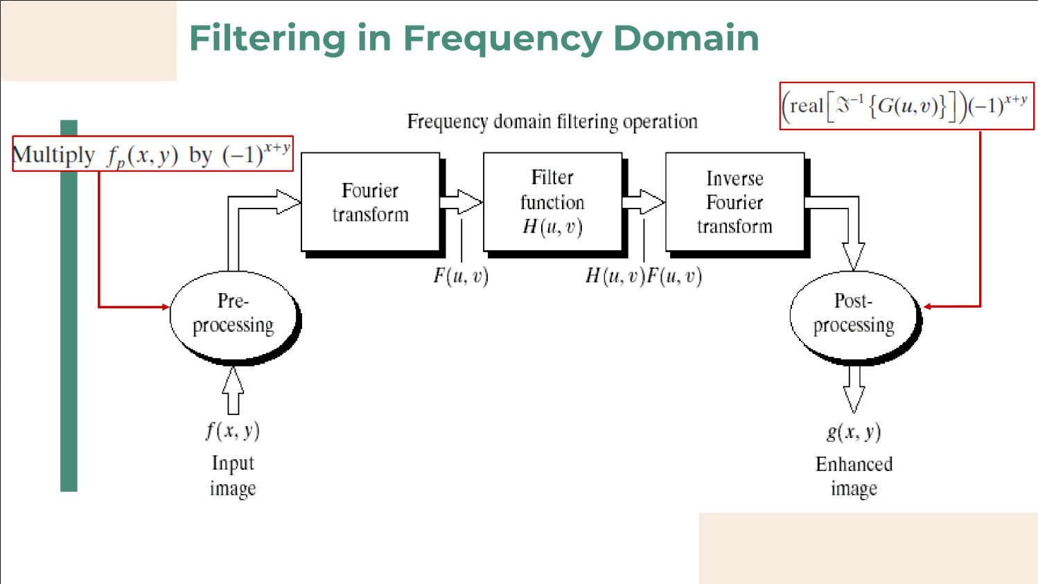
The complete filtering pipeline involves five steps:

Pre-processing: Center the Transform by multiplying the input image $f (x, y)$ by $(- 1)^{x + y}$ , then compute its Discrete Fourier Transform (DFT), $F (u, v)$ .
Filtering: Multiply the centered DFT by the filter function $H (u, v)$ to get $G (u, v)$ .
$G (u, v) = F (u, v) H (u, v)$
Inverse Transform: Compute the Inverse DFT of the filtered result $G (u, v)$ .
Extract Real Part: Take the real part of the inverse transform result.
Post-processing: Un-center the image by multiplying it again by $(- 1)^{x + y}$ to get the final enhanced image $g (x, y)$ .

Pasted image 20260402005015.png

Understanding Image Frequencies

To choose the right filter, you have to understand what frequencies represent in an image:

Low Frequencies: Represent areas where gray levels change very little over distance, such as smooth backgrounds or skin textures.
High Frequencies: Represent areas with large, rapid changes in gray levels, such as sharp edges, fine details, and noise.

The Two Main Filtering Categories

Filters are categorized by which frequencies they allow to "pass" through:

Lowpass Filters (Smoothing): These allow low frequencies to pass while attenuating (reducing) high frequencies. Because high frequencies contain edges and noise, reducing them results in a blurred or smoothed image. They are useful for joining broken text characters or smoothing out skin blemishes.
Highpass Filters (Sharpening): These allow high frequencies to pass while attenuating low frequencies. This drops the smooth background and highlights edges and fine details. Mathematically, a highpass filter is simply the exact reverse of a lowpass filter: $H_{H P} (u, v) = 1 - H_{L P} (u, v)$ .

Comprehensive Comparison of Filter Shapes

Whether you are smoothing (Lowpass) or sharpening (Highpass), there are three primary mathematical shapes used for the filter function $H (u, v)$ . The main differentiator between them is how they handle the "cutoff frequency" $D_{0}$ (the distance from the center where the filter starts blocking frequencies).

Here is a complete comparison of the three methods:

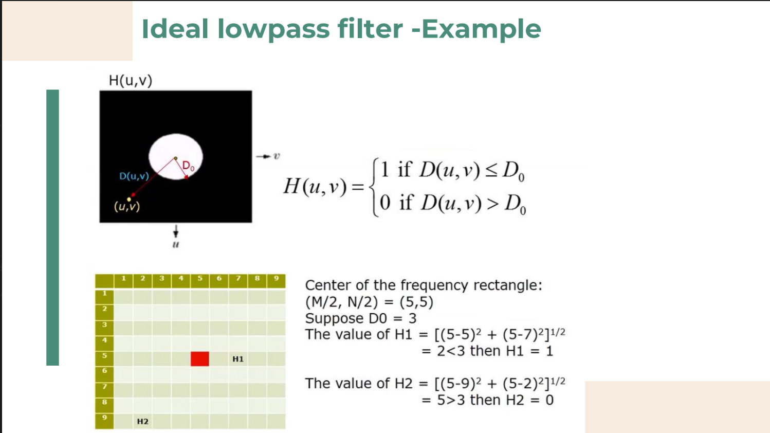
Feature	Ideal Filter (ILPF / IHPF)	Butterworth Filter (BLPF / BHPF)	Gaussian Filter (GLPF / GHPF)
Cutoff Style	Extremely sharp, abrupt cutoff at distance $D_{0}$ .	Smooth transition, controlled by an order parameter $n$ . more on it here	Very smooth, gradual exponential decay.
Mathematical Definition (Lowpass)	$$H(u,v) = \begin{cases} 1 & \text{if } D(u,v) \le D_0 \ 0 & \text{if } D(u,v) > D_0 \end{cases}$$	$$H(u,v) = \frac{1}{1 + [D(u,v)/D_0]^{2n}}$$	$$H(u,v) = e^{-D^2(u,v) / 2D_0^2}$$
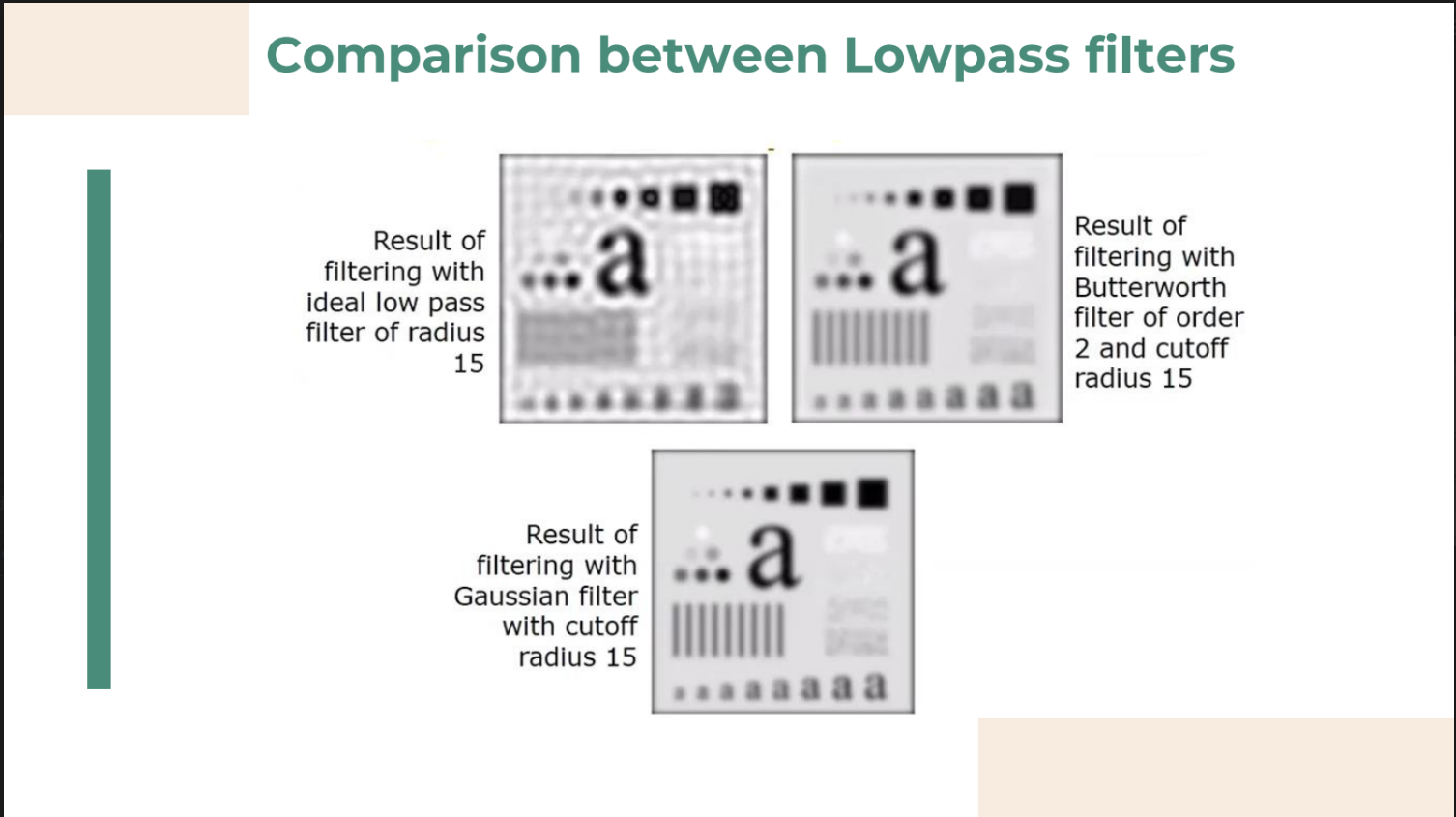
Ringing Effect	Severe. The sharp cutoff creates distinct, visible ripples (ringing) around edges in the filtered image.	Variable. Ringing depends on order $n$ . It approaches the Ideal filter at high orders, and the Gaussian filter at low orders.	None. The smooth transition guarantees that absolutely no ringing artifacts will appear.
Practical Usage	Rarely used in practical applications due to the severe ringing artifacts.	Highly versatile. An order of $n = 2$ is considered the best compromise, offering effective filtering with almost imperceptible ringing.	Highly practical, especially when any form of artifacting (ringing) is unacceptable, such as in medical imaging.
Visual Result	Heavy blurring/sharpening but with noticeable, distracting "echoes" around sharp objects.	Balanced blurring/sharpening. Edges remain relatively clean without excessive echoing.	Very smooth blurring/sharpening, but requires a lower $D_{0}$ to achieve the same level of sharpness/blur as Butterworth.

For Highpass, just 1 - Lowpass, and for Butterworth just flip the ratio

Pasted image 20260402005701.png

Pasted image 20260402010404.png