• What it is: Unlike spatial filtering which alters pixel values directly, this technique processes images by manipulating their frequency components. It uses the Fourier Transform to convert an image from the spatial domain to the frequency domain.
  
  

• Why we use it: It is highly efficient for specific operations like noise removal, sharpening, and blurring. It allows us to target specific image contents: smooth areas correspond to low frequencies, while edges and details correspond to high frequencies.
  
  

• Spatial vs. Frequency:

  • Spatial Domain: Works with pixel intensities directly (e.g., applying convolution masks like Gaussian blur). It is intuitive but can be computationally heavy for large filters.
    
    
  • Frequency Domain: Represents the image as combinations of sine and cosine waves. Filtering here is done via simple multiplication instead of convolution, making it significantly faster for large filter kernels.
    
    

• Practical Example: The slides demonstrate periodic noise removal using an image of the moon from NASA. The original image suffers from sinusoidal interference. By viewing the magnitude of the Fourier transform, the interference appears as distinct "bursts of energy". A mask is applied to eliminate these bursts, and the inverse Fourier transform reconstructs a clean, filtered image.

The Big Idea & Historical Context (Slides 6-11)

• History: Jean Baptiste Joseph Fourier (born 1768 in France) introduced these concepts in his 1822 work, "The Analytic Theory of Heat". Though largely ignored at publication, it became a foundational mathematical theory for modern engineering.
  
  

• Fourier Series & Transform:

  • Series: Any periodic function can be expressed as a sum of sines and cosines of different frequencies.
    
    
  • Transform: Even non-periodic functions (with finite area) can be expressed as the integral of sines or cosines multiplied by a weighting function.
    
    

• The Prism Analogy: Just as a glass prism separates light into its component colors (frequencies), the Fourier Transform acts as a "mathematical prism" that separates spatial data $f(x,y)$ into frequency data $F(u,v)$.

• Properties: Low frequencies cluster near the center (representing overall structure), while high frequencies spread to the outer edges (representing fine details and noise). Importantly, the image can be completely recovered without information loss via the Inverse Fourier Transform.

The Mathematics of Fourier Transform (Slides 12-28)

The lecture breaks down the transform into four distinct cases:

The cases are divided by Dimensionality (1-D vs. 2-D) and the Type of Signal (Continuous vs. Discrete).

The Core Difference: Forward vs. Inverse

Before diving into the cases, notice the mathematical pattern that applies to all of them:

• Forward Transform ($f\to F$): Always uses a negative sign in the exponential ($-j$). It moves from spatial data to frequency data.

• Inverse Transform ($F\to f$): Always uses a positive sign in the exponential ($+j$). It moves from frequency data back to spatial data.

Case 1: 1-D Continuous Signals

Used for infinite, continuous analog signals over time or space (like a continuous audio wave or an analog voltage signal). Because the signal is continuous, the equations rely on integration.

• Forward Transform:

  $$F(u)={\int }_{-\mathrm{\infty }}^{\mathrm{\infty }}f(x)e^{-j2\pi ux}dx$$

• Inverse Transform:

  $$f(x)={\int }_{-\mathrm{\infty }}^{\mathrm{\infty }}F(u)e^{j2\pi ux}du$$

• Example Application: Analyzing the frequency spectrum of a continuous sine wave generated by an analog synthesizer.

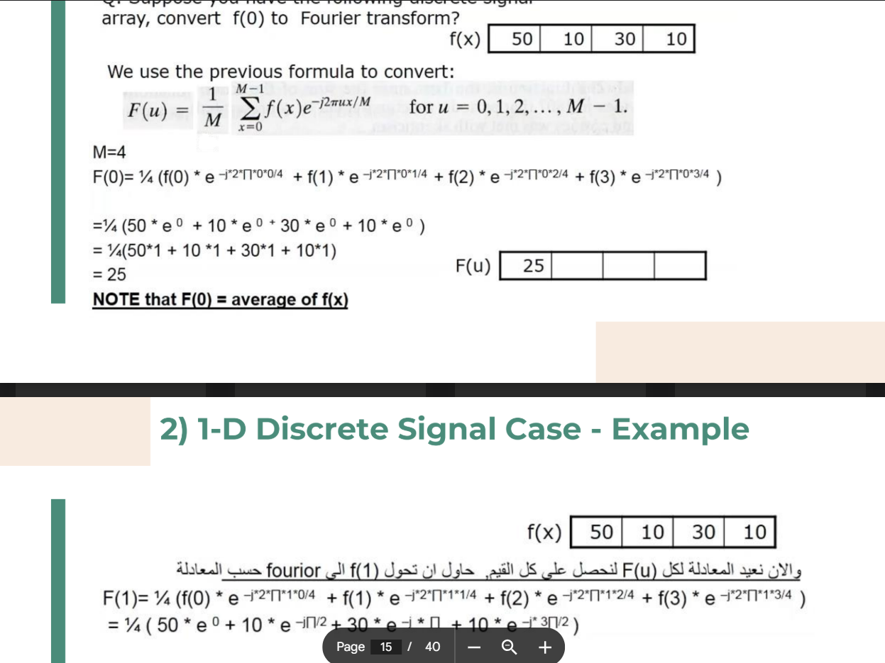
Case 2: 1-D Discrete Signals (1D DFT)

Used for sampled, digital signals (like a digital audio file or a 1-D array of sensor data). Because the data is discrete and finite (length $M$), the integrals are replaced by summations.

• Forward Transform:

  $$F(u)=\frac{1}{M}\sum _{x=0}^{M-1}f(x)e^{-j2\pi ux/M}$$

• Inverse Transform:

  $$f(x)=\sum _{u=0}^{M-1}F(u)e^{j2\pi ux/M}$$

• Example Calculation: Let's say you have a 1-D array of pixel intensities: $f(x)=[50,10,30,10]$ where $M=4$.

  To find the DC component $F(0)$, you plug $u=0$ into the forward equation. Since $e^0=1$, the math simplifies to $F(0)=\frac{1}{4}(50+10+30+10)=25$.

  Tip for calculating the higher frequencies like $F(1)$ by hand: You have to expand the $e^{-j\dots }$ term using Euler's formula ($\cos -j\sin$). You can compute these complex numbers efficiently during an exam by switching a standard scientific calculator, like the Casio fx-991ES Plus, into CMPLX mode (Mode 2) to handle the real and imaginary ($i$) parts directly without manually calculating the sines and cosines every time.

Case 3: 2-D Continuous Signals

An extension of Case 1 into two dimensions. This is purely theoretical in modern digital computing but is foundational for optical physics.

• Forward Transform:

  $$F(u,v)={\int }_{-\mathrm{\infty }}^{\mathrm{\infty }}{\int }_{-\mathrm{\infty }}^{\mathrm{\infty }}f(x,y)e^{-j2\pi (ux+vy)}dxdy$$

• Inverse Transform:

  $$f(x,y)={\int }_{-\mathrm{\infty }}^{\mathrm{\infty }}{\int }_{-\mathrm{\infty }}^{\mathrm{\infty }}F(u,v)e^{j2\pi (ux+vy)}dudv$$

• Example Application: How a physical glass lens bends continuous light waves. The mathematical transformation that happens to light as it passes through a lens can be perfectly modeled by these double integrals.

Case 4: 2-D Discrete Signals (2D DFT)

This is the most critical case for Digital Image Processing. It applies to 2-D matrices of finite discrete data (an image with $M$ rows and $N$ columns).

• Forward Transform:

  $$F(u,v)=\frac{1}{MN}\sum _{x=0}^{M-1}\sum _{y=0}^{N-1}f(x,y)e^{-j2\pi (ux/M+vy/N)}$$

• Inverse Transform:

  $$f(x,y)=\sum _{u=0}^{M-1}\sum _{v=0}^{N-1}F(u,v)e^{j2\pi (ux/M+vy/N)}$$

• Example Application: Processing a digital photograph. Imagine a tiny $2\times 2$ pixel image matrix. To find $F(1,1)$, you must loop through all four pixels ($x,y$ coordinates: 0,0; 0,1; 1,0; 1,1), multiplying each pixel's intensity by the complex exponential, and summing the results.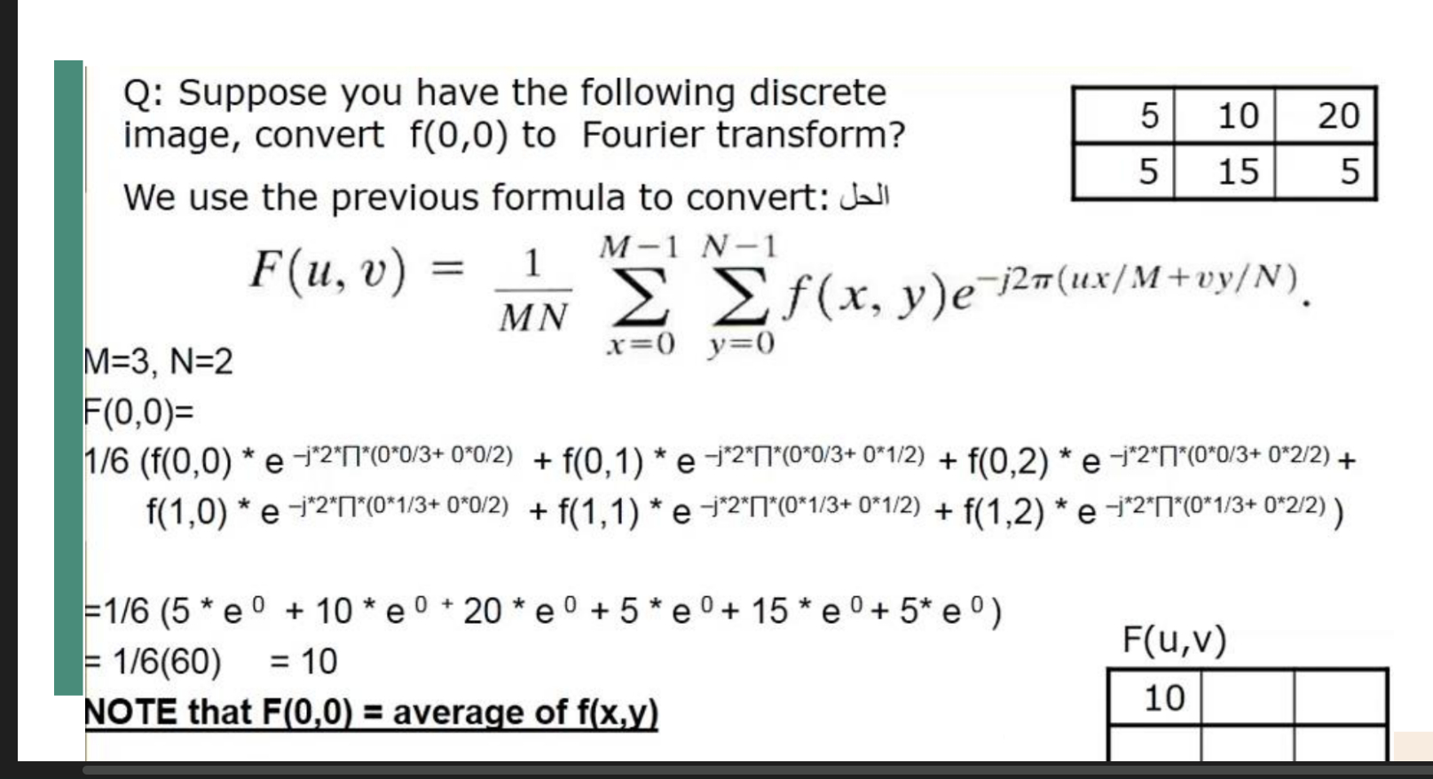

  
  

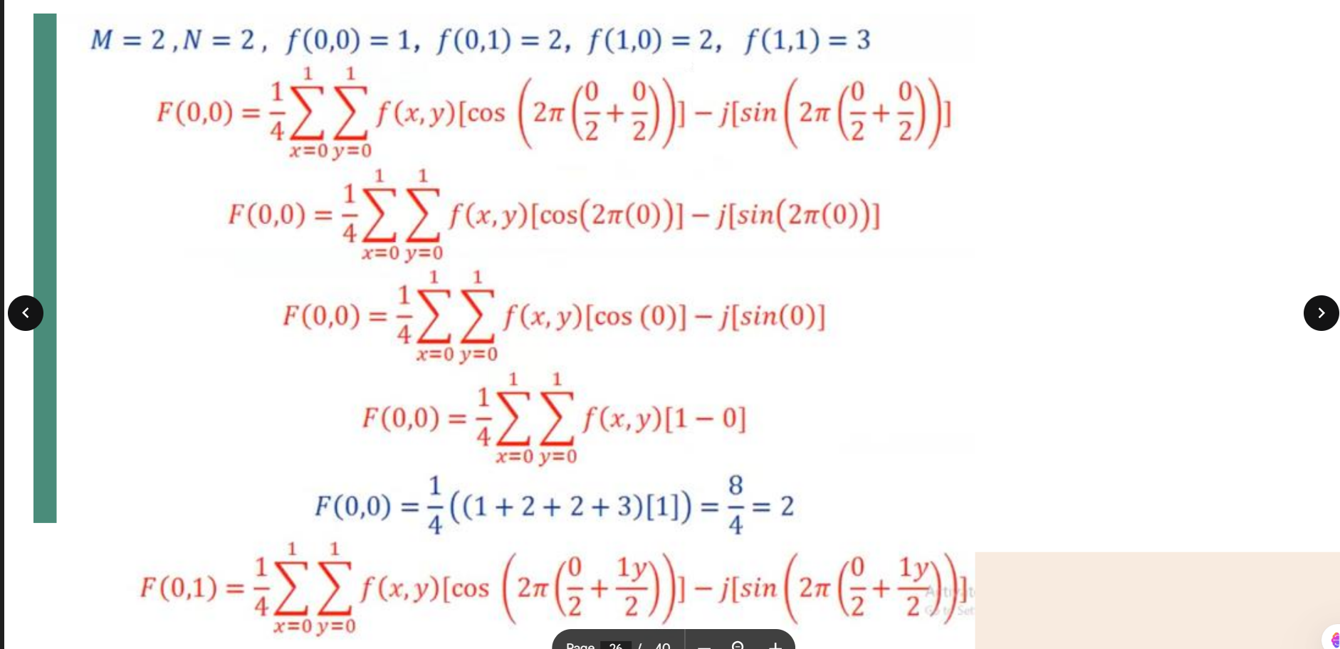
Image Spectra and The Filtering Pipeline (Slides 29-36)

• Spectrum Characteristics: The $F(0,0)$ value is typically the largest component of the image, while other frequencies diminish rapidly. Because the magnitude drops off so quickly, we display the spectrum using a log transformation: $log(1+|F(u,v)|)$.

• The Filtering Pipeline:

  1. Compute the DFT $F(u,v)$ of the input image $f(x,y)$.
     
     
  2. Multiply $F(u,v)$ by a chosen filter function $H(u,v)$.
     
     
  3. Compute the Inverse DFT of the result to get the enhanced image $g(x,y)$.

• Magnitude vs. Phase: The Fourier Transform outputs a complex number, $$F(u,v) = R(u,v) + jI(u,v)$$

  • Magnitude (Amplitude): Calculated as $|F(u,v)|=[R^2(u,v)+I^2(u,v){]}^{1/2}$. It dictates the size/height of the peak (intensities) and reveals the presence and boundaries of features.
    
    
  • Phase: Calculated as $\varphi (u,v)=ta{n}^{-1}[\frac{I(u,v)}{R(u,v)}]$. It acts as a measure of displacement, encoding exactly where objects are located in the image.
    
    
  • Because phase is crucial for maintaining the spatial coherence of the image, frequency domain filtering usually only manipulates the amplitude spectrum, leaving the phase untouched.

Shifting & Fourier Properties (Slides 37-40)

• Shifting the Origin: To make the Fourier spectrum easier to analyze (putting the low frequencies in the center), we multiply the input image $f(x,y)$ by $(-1{)}^{x+y}$ before applying the transform.
  
  
• Properties: Operations applied in the spatial domain have direct geometric impacts in the frequency domain. The slides visually demonstrate how image rotation, linear shifting, and scaling alter the resulting Fourier spectrum pattern.