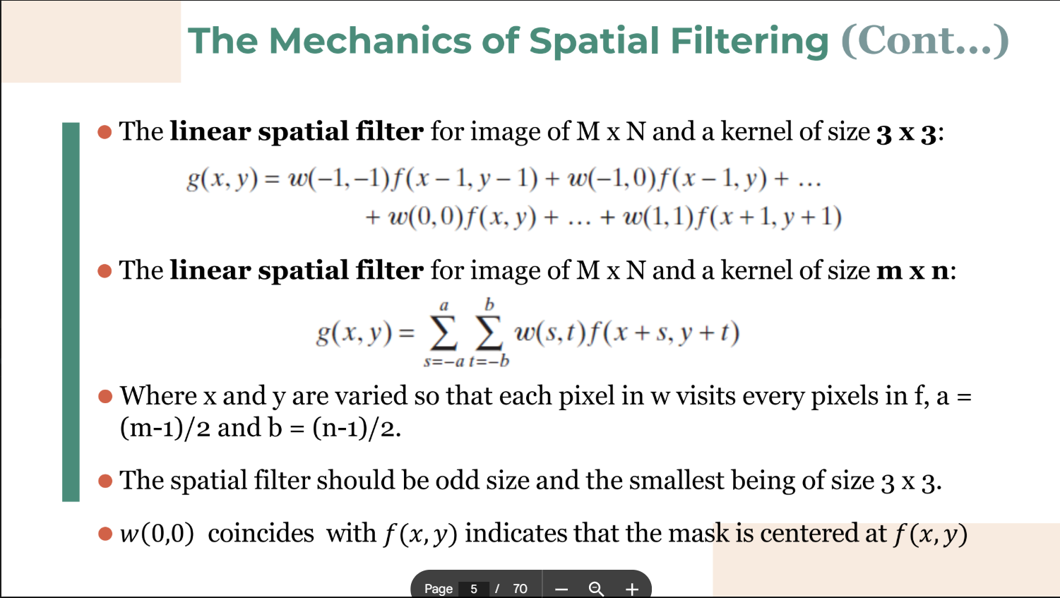
Lecture 5 - Intensity Transformation and Spatial Filtering - Ch3

Mechanics of Spatial Filtering

While point processing (intensity transformation) operates on a $1 \times 1$ neighborhood, spatial filtering uses a larger neighborhood (e.g., a $3 \times 3$ mask, kernel, or window).

The Process: The spatial filter mask is moved from point to point across the image. At each coordinate $(x, y)$ , a predefined operation is performed on the image pixels within the neighborhood, generating a new pixel value for the center coordinate.
Categories:
1. Linear Spatial Filtering: Involves multiplying pixels by corresponding mask coefficients and summing the results (Convolution/Correlation).
2. Nonlinear Spatial Filtering: Operates based on ranking or ordering pixel values within the neighborhood.

Pasted image 20260401230549.png

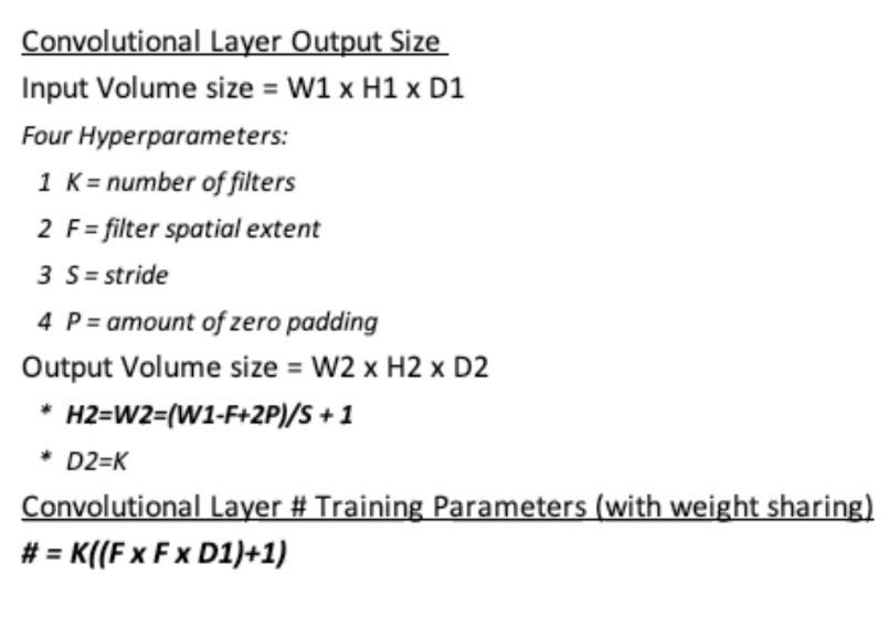
Convolution Output Size Formula

When applying a filter, the spatial dimensions of the output image can be calculated using the following formula:

O = \frac{W - K + 2 P}{S} + 1

$O$ : Output dimension (Width or Height)
$W$ : Input dimension
$K$ : Filter (Kernel) size
$P$ : Padding applied to the input
$S$ : Stride (step size of the filter)

Pasted image 20260401230312.png

What Happens at the Borders?

The mask falls outside the edge!
Solutions?
- Ignore the edges: The resultant image is smaller than the original
- Pad with zeros: Introducing unwanted artifacts
- Repeat rows and columns: Pad with adjacent rows and columns

2. Smoothing Spatial Filters

Smoothing filters are used for blurring (a preprocessing step to remove small details or bridge gaps in lines) and for noise reduction.

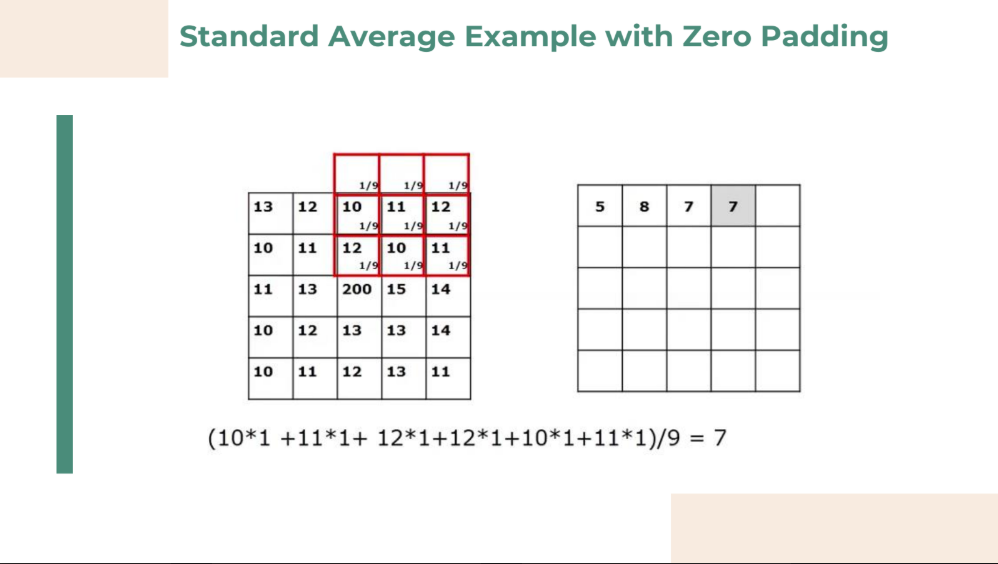
A. Linear Smoothing Filters (Averaging)

These filters replace the value of every pixel with the average of the intensity levels in its neighborhood.

Effect: Reduces "sharp" transitions in intensities. Because random noise typically consists of sharp transitions, averaging effectively reduces noise. However, edges are also sharp transitions, so this causes undesirable edge blurring.
Characteristics:
1. The elements of the mask must be positive.
2. Sum of mask elements is 1
Types of Masks:
- Box Filter: All coefficients in the mask are equal (typically $1$ ). The sum is divided by the total number of pixels in the mask (e.g., $\frac{1}{9}$ for a $3 \times 3$ mask).
- Weighted Average Filter: Pixels closer to the center of the mask are given higher weight (importance) than those further away, which helps reduce blurring compared to a standard box filter.

Pasted image 20260331023035.png

B. Order-Statistic Filters (Nonlinear)

These filters replace the center pixel based on the ordering (ranking) of the pixels in the image area encompassed by the filter.

Median Filter: Replaces the value of a pixel with the median of the intensity levels in the neighborhood.
- Application: Provides excellent noise-reduction for impulse noise (salt-and-pepper noise) with considerably less blurring than linear smoothing filters.
Max Filter: Replaces the pixel with the maximum value in the neighborhood. Useful for finding the brightest points (removes "pepper" noise).
Min Filter: Replaces the pixel with the minimum value in the neighborhood. Useful for finding the darkest points (removes "salt" noise).

3. Sharpening Spatial Filters

The objective of sharpening is to highlight transitions in intensity (edges, boundaries). Because smoothing is achieved by spatial averaging (integration), sharpening is achieved by spatial differentiation.

Characteristics:
- The elements of the mask contain both positive and negative weights.
- Sum of the mask weights is 0

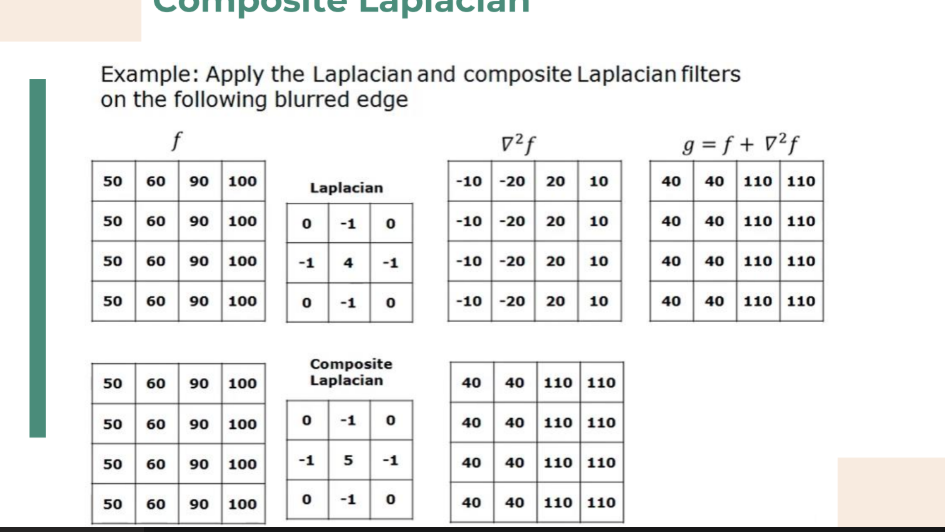
A. The Laplacian (Second Derivative)

The Laplacian is an isotropic (rotation-invariant) operator that calculates the second derivative of the image to find rapid changes in intensity.

Mathematical Definition:

\nabla^{2} f = \frac{\partial^{2} f}{\partial x^{2}} + \frac{\partial^{2} f}{\partial y^{2}}

Discrete Approximation Masks:

Common $3 \times 3$ masks for the Laplacian include a center value of $- 4$ (with $1$ s on the top, bottom, left, and right) or a center of $- 8$ (with $1$ s in all surrounding cells).

Image Enhancement with the Laplacian:

Because the Laplacian highlights edges but zeroes out flat areas (losing the background), the sharpened image is usually added back to the original image to restore the background information.

g (x, y) = f (x, y) + c [\nabla^{2} f (x, y)]

(Where $c$ depends on the center coefficient of the mask, negative center corresponds to c = 1, and vice versa).

Screenshot 2026-03-30 172816.png

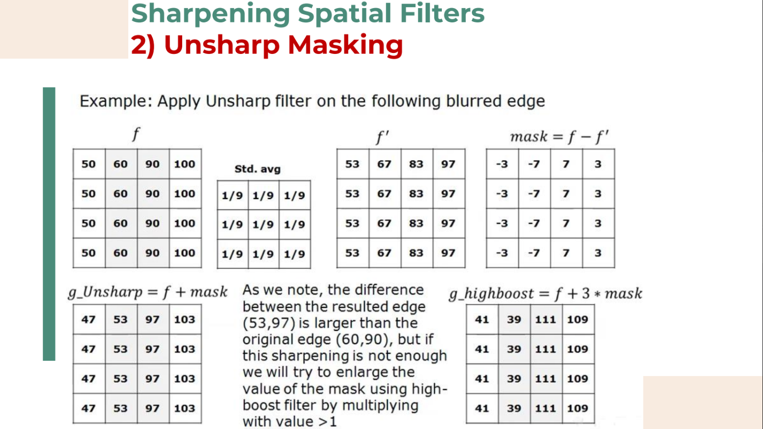
B. Unsharp Masking & Highboost Filtering

This is a classic technique used in the publishing industry, consisting of three steps:

Blur the original image: $\bar{f} (x, y)$
Subtract the blurred image from the original to create a mask:
$g_{m a s k} (x, y) = f (x, y) - \bar{f} (x, y)$
Add the mask back to the original image:
$g (x, y) = f (x, y) + k \cdot g_{m a s k} (x, y)$

$k = 1$ : Unsharp masking.
$k > 1$ : Highboost filtering (increases the contribution of the edges).

Pasted image 20260401233437.png

C. The Gradient (First Derivative)

First derivatives are primarily used to extract edges (rather than just enhance the whole image). The gradient of an image $f$ at $(x, y)$ is a vector:

\nabla f = [\begin{matrix} G_{x} \\ G_{y} \end{matrix}] = [\begin{matrix} \frac{\partial f}{\partial x} \\ \frac{\partial f}{\partial y} \end{matrix}]

Gradient Magnitude:

To calculate the strength of the edge, we find the magnitude. In image processing, this is often approximated using absolute values for computational speed:

M (x, y) \approx | G_{x} | + | G_{y} |

Common Gradient Operators:

Roberts Cross-Gradient: Uses $2 \times 2$ masks to compute diagonal differences.
Sobel Operators: Uses $3 \times 3$ masks. They compute $G_{x}$ (horizontal changes) and $G_{y}$ (vertical changes). Using a $3 \times 3$ neighborhood provides a slight smoothing effect, making the Sobel operators less sensitive to noise than the Roberts operators.

Too see full comparison and summary for Ch3, here