Lecture 9 - Image Segmentation

Image Segmentation Fundamentals

Image segmentation is a fundamental process in computer vision that subdivides an image into its constituent regions or objects. It is commonly defined as the process of grouping together pixels that share similar attributes, partitioning the image into non-intersecting, homogeneous regions. Segmentation is typically the first phase in pattern recognition and object isolation problems.

The typical image classification cycle follows a distinct pipeline:

Image Segmentation: Extracts the Region of Interest (ROI) from the original image.
Feature Extraction: Generates a feature vector from the segmented region.
Classification: Determines the object type based on the extracted features.

Approaches to Image Segmentation

The primary goal of segmentation is to isolate individual objects within an image. There are two fundamental approaches to achieving this:

Discontinuity (Boundary-based): This approach partitions an image based on abrupt changes in intensity, such as points, lines, and edges.
Similarity (Region-based): This approach partitions an image into regions that are similar according to predefined criteria, using techniques like thresholding, region growing, and region splitting and merging.

Detection of Discontinuities

To find discontinuities (points, lines, or edges), the most common method involves passing a small mask (or filter) over the image. The mask determines the specific type of discontinuity being targeted. The response of the mask at any given point is the sum of the products of the mask coefficients and the corresponding image pixels: $Z = \sum_{k = 1}^{9} w_{k} z_{k}$ .

Point Detection

Point detection utilizes a mask where the coefficients sum to zero, ensuring that the response is zero in areas of constant gray levels. A point is detected if the absolute value of the response is greater than or equal to a non-negative threshold: $| R | \geq T$ .

The standard point detection mask features an 8 in the center pixel and -1 for all surrounding pixels.

Line Detection

Line detection uses specific masks designed to extract lines that are one pixel thick in a particular direction. In digital images, straight lines are typically evaluated in horizontal, vertical, or diagonal directions.

Horizontal Mask: A row of 2s in the middle, surrounded by -1s.
Vertical Mask: A column of 2s in the middle, surrounded by -1s.
Diagonal Masks: Consist of 2s arranged diagonally, with -1s filling the rest of the mask.

Edge Detection

An edge is a set of connected pixels lying on the boundary between two regions. Detecting edges can be challenging because derivative-based edge detectors are extremely sensitive to noise, and actual edges often resemble a "ramp" profile rather than an ideal step profile due to blurring.

First-Order Derivatives (Gradient)

The first derivative of an image identifies edges by finding the maximum rate of change in intensity. The gradient of an image $f (x, y)$ is a vector $\nabla f$ containing the partial derivatives in the x and y directions.

Magnitude: Indicates the strength of the edge, calculated as $m a g (\nabla f) = [G_{x}^{2} + G_{y}^{2}]^{1 / 2}$ .
Direction: Perpendicular to the edge direction, calculated as $α (x, y) = t a n^{- 1} (\frac{G_{y}}{G_{x}})$ .

Several operators are used to compute these gradients:

Roberts Cross-Gradient Operators: Utilize a simple $2 \times 2$ matrix configuration.
Prewitt Operators: Use a $3 \times 3$ matrix (e.g., -1, 0, 1 across columns or rows) to find horizontal and vertical edges.
Sobel Operators: Similar to Prewitt but place a higher weight (2 and -2) on the center pixels to provide some smoothing.

To output a binary segmentation matrix, a threshold is applied to the final gradient magnitude. Due to the high level of detail sometimes captured by these masks, images are often smoothed prior to edge detection.

Second-Order Derivatives (Laplacian)

The second derivative finds edges by searching for "zero crossings"—the point where the second derivative changes sign, indicating the midpoint of the edge ramp. The Laplacian of a 2D function is the sum of its second unmixed partial derivatives.

Laplacian Masks: Common implementations use a $3 \times 3$ matrix with a 4 or an 8 in the center pixel and -1s in the surrounding neighbor pixels.
Zero Crossing: A crossing occurs if adjacent pixels in the Laplacian result have different signs.

Laplacian of a Gaussian (LoG)

Because the Laplacian is highly sensitive to noise, it is rarely used alone. Instead, it is combined with a Gaussian smoothing filter, creating the Laplacian of a Gaussian, also known as the Mexican hat function. This method uses the Gaussian component for noise removal and the Laplacian component for edge detection.

Edge Linking and Boundary Detection

After detecting edge points, local processing is used to link them together to form continuous boundaries. Adjacent edge points are linked if they share similar properties within a local neighborhood.

Two primary criteria must be met to link a pixel at $(x_{0}, y_{0})$ to a neighboring pixel at $(x, y)$ :

Magnitude Similarity: The difference in their gradient magnitudes must be less than or equal to a non-negative threshold: $| \nabla f (x, y) - \nabla (x_{0}, y_{0}) | \leq E$ .
Direction Similarity: The difference in their gradient angles must be less than an angle threshold: $| α (x, y) - α (x_{0}, y_{0}) | < A$ .

Technique	Category	Kernel / Mask	Key Characteristics & Methodology
Point Detection	Discontinuity	$[\begin{matrix} - 1 & - 1 & - 1 \\ - 1 & 8 & - 1 \\ - 1 & - 1 & - 1 \end{matrix}]$	Detects isolated points. The coefficients sum to zero. A point is detected if the absolute response exceeds a threshold ($
Horizontal Line	Discontinuity	$[\begin{matrix} - 1 & - 1 & - 1 \\ 2 & 2 & 2 \\ - 1 & - 1 & - 1 \end{matrix}]$	Extracts straight lines that are one pixel thick in the horizontal direction.
Vertical Line	Discontinuity	$[\begin{matrix} - 1 & 2 & - 1 \\ - 1 & 2 & - 1 \\ - 1 & 2 & - 1 \end{matrix}]$	Extracts straight lines that are one pixel thick in the vertical direction.
Diagonal Line (+45°)	Discontinuity	$[\begin{matrix} 2 & - 1 & - 1 \\ - 1 & 2 & - 1 \\ - 1 & - 1 & 2 \end{matrix}]$	Extracts straight lines that are one pixel thick in the positive diagonal direction.
Diagonal Line (-45°)	Discontinuity	$[\begin{matrix} - 1 & - 1 & 2 \\ - 1 & 2 & - 1 \\ 2 & - 1 & - 1 \end{matrix}]$	Extracts straight lines that are one pixel thick in the negative diagonal direction.
Roberts Cross	Edge (1st Order)	$G_{x} = [\begin{matrix} - 1 & 0 \\ 0 & 1 \end{matrix}]$ $G_{y} = [\begin{matrix} 0 & - 1 \\ 1 & 0 \end{matrix}]$	Computes the 2D spatial gradient on an image to find maximum rates of intensity change using a simple 2x2 neighborhood.
Prewitt Operator	Edge (1st Order)	$G_{x} = [\begin{matrix} - 1 & - 1 & - 1 \\ 0 & 0 & 0 \\ 1 & 1 & 1 \end{matrix}]$ $G_{y} = [\begin{matrix} - 1 & 0 & 1 \\ - 1 & 0 & 1 \\ - 1 & 0 & 1 \end{matrix}]$	Calculates gradient magnitude and direction. It is highly sensitive to noise, often requiring prior image smoothing.
Sobel Operator	Edge (1st Order)	$G_{x} = [\begin{matrix} - 1 & - 2 & - 1 \\ 0 & 0 & 0 \\ 1 & 2 & 1 \end{matrix}]$ $G_{y} = [\begin{matrix} - 1 & 0 & 1 \\ - 2 & 0 & 2 \\ - 1 & 0 & 1 \end{matrix}]$	Provides a localized smoothing effect by giving higher weight (2 and -2) to the center pixels, making it slightly more robust to noise than Prewitt.
Laplacian (8-neighbor)	Edge (2nd Order)	$\nabla^{2} = [\begin{matrix} - 1 & - 1 & - 1 \\ - 1 & 8 & - 1 \\ - 1 & - 1 & - 1 \end{matrix}]$	Detects edges by locating "zero crossings" (where the 2nd derivative changes sign). Extremely sensitive to noise and rarely used alone.
Laplacian of a Gaussian (LoG)	Edge (2nd Order)	Gaussian filter followed by Laplacian	Uses the Gaussian component to remove noise and blur the image before the Laplacian component detects the edges via zero crossings (Mexican hat function).
Local Processing	Edge Linking	Local neighborhood analysis (e.g., 3x3 or 5x5)	Links detected edge pixels if they have similar gradient magnitudes

Pasted image 20260413233224.png

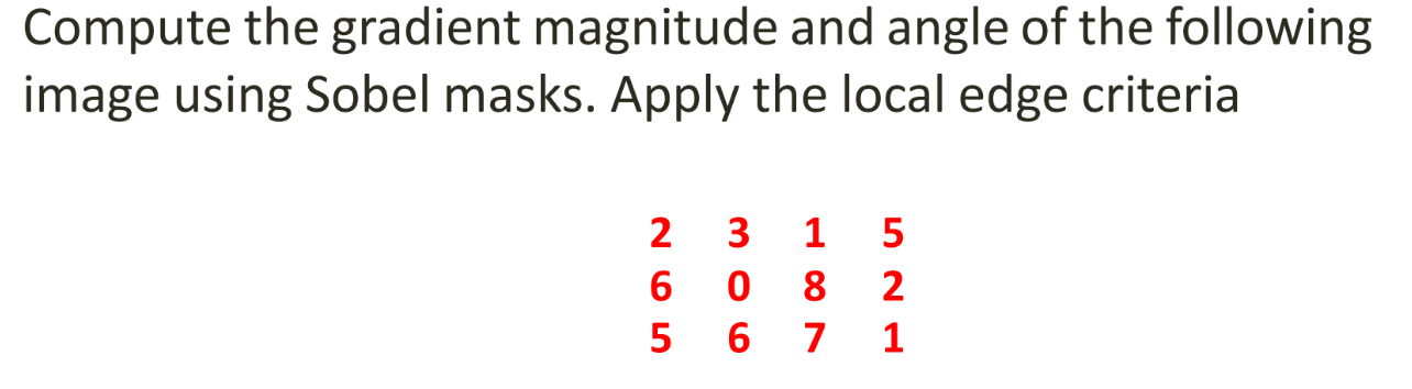
1. Compute Gradient Matrices ( $d_{x}$ and $d_{y}$ )

First, we apply the horizontal and vertical Sobel masks to the image using zero-padding for the boundaries.

According to the slides, the Sobel masks used are: $d_{x} = [\begin{matrix} - 1 & - 2 & - 1 \\ 0 & 0 & 0 \\ 1 & 2 & 1 \end{matrix}]$ $d_{y} = [\begin{matrix} - 1 & 0 & 1 \\ - 2 & 0 & 2 \\ - 1 & 0 & 1 \end{matrix}]$

Applying these masks to the image yields the following gradient matrices:

$d_{x}$ Matrix:

$[\begin{matrix} 12 & 14 & 18 & 12 \\ 15 & 9 & 11 & - 2 \\ - 14 & - 12 & - 18 & - 12 \end{matrix}]$

$d_{y}$ Matrix:

$[\begin{matrix} 6 & 0 & 6 & - 10 \\ 9 & 5 & 1 & - 24 \\ 12 & - 8 & 6 & - 22 \end{matrix}]$

2. Compute Gradient Magnitude

The gradient magnitude is calculated using the formula $\nabla f = \sqrt{d_{x}^{2} + d_{y}^{2}}$ . The slides provide this

computed matrix as: Magnitude Matrix: $[\begin{matrix} 13.4 & 14.0 & 18.9 & 15.6 \\ 12.72 & 15.8 & 11.04 & 24.08 \\ 16.97 & 15.23 & 19.69 & 25.05 \end{matrix}]$

3. Compute Gradient Angle

The angle of the gradient is perpendicular to the edge direction and is calculated using the formula $α (x, y) = \tan^{- 1} (\frac{d_{y}}{d_{x}})$ .

For example, calculating the angle for the top-left pixel (where $d_{x} = 12$ and $d_{y} = 6$ ):

$α (0, 0) = \tan^{- 1} (\frac{6}{12}) = 0.464 radians$

Applying this to every pixel gives us the Angle Matrix (in radians):

$[\begin{matrix} 0.464 & 0.000 & 0.322 & - 0.695 \\ 0.540 & 0.507 & 0.090 & 1.488 \\ - 0.709 & - 0.588 & - 0.322 & 1.071 \end{matrix}]$

4. Apply Local Edge Linking Criteria

To link edges, we evaluate a local neighborhood against a specific "seed" pixel $(x_{0}, y_{0})$ . A neighboring pixel $(x, y)$ is linked to the seed pixel if both of the following criteria are met:

Magnitude Similarity: $| \nabla f (x, y) - \nabla f (x_{0}, y_{0}) | \leq E$ (where $E$ is a non-negative threshold).
Angle Similarity: $| α (x, y) - α (x_{0}, y_{0}) | < A$ (where $A$ is a non-negative angle threshold).

Because the problem statement in Example-3 does not specify the seed pixel or the thresholds $E$ and $A$ , just assume any two numbers and calculate the differences, if the magnitude of diff is less than or equal to thresholds, turn 0 to 1.