While the first half focused on finding local discontinuities (points, lines, and edges), this half shifts to piecing those local features into global shapes and grouping pixels based on similarity.

1. Global Processing: The Hough Transform

Local edge linking (like the neighborhood magnitude/angle checks we did previously) can sometimes struggle to connect fragmented edges into meaningful shapes. If the goal is to detect straight, continuous structures—like tracking lane boundaries for highway traffic analysis—we need a global perspective. The Hough Transform is a technique used to find edge points that lie along a specific mathematical shape, most commonly straight lines.

The Mathematical Concept

Instead of looking at the image in the standard Cartesian $xy$-plane, the Hough Transform maps points into a "Parameter Space".

Initially, you might think to use the standard line equation $y=ax+b$ to map to an $ab$-plane. However, vertical lines have an infinite slope ($a=\mathrm{\infty }$), which breaks the math. To solve this, the algorithm uses a polar coordinate representation:

• $\rho$ is the perpendicular distance from the origin to the line.

• $\theta$ is the angle of that perpendicular line (ranging from $0$ to $2\pi$).

The Accumulator Algorithm

1. Initialize: Create a 2D matrix (an accumulator array) where the rows represent quantized values of $\rho$ and columns represent quantized values of $\theta$. Set all cells to zero.

2. Transform: For every edge pixel $(x_k,y_k)$ found in your image, loop through every possible angle $\theta$ and calculate the resulting $\rho$ using the polar equation.

3. Vote: Round $\rho$ to the nearest index and increment that $(\rho ,\theta )$ cell in the accumulator by 1.

4. Extract: A single point in the $xy$-plane becomes a sinusoidal curve in the $\rho \theta$-plane. When multiple curves intersect at the exact same $(\rho ,\theta )$ cell, it creates a "peak" in the accumulator. This peak represents a strong line in the original image.

The goal of this example is to take a binary image containing edge pixels and map them into the Hough parameter space ($\rho ,\theta$) to detect straight lines.

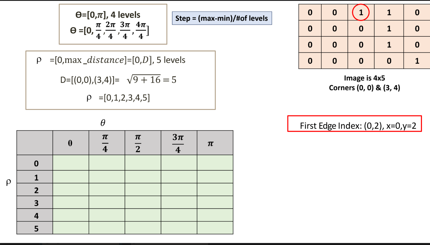
1. Setting Up the Image and Coordinate System

The example begins with a $4\times 5$ binary image matrix where the 1s represent detected edge pixels.

• Coordinate System: The corners of the image are defined as $(0,0)$ at the top-left and $(3,4)$ at the bottom-right. This indicates that $x$ represents the row index and $y$ represents the column index.

• Maximum Distance ($D$): The maximum possible perpendicular distance from the origin to any line in this image is the diagonal distance, calculated as $D=\sqrt{3^2+4^2}=5$.

• Edge Points: Based on the provided matrix, the edge points $(x,y)$ are located at:

  • $(0,2)$

  • $(0,3)$

  • $(1,3)$

  • $(2,3)$

  • $(3,4)$

2. Parameter Space Quantization

To create the 2D accumulator array, the continuous parameters $\rho$ and $\theta$ must be quantized into discrete bins.

• Angle ($\theta$): The slides specify ranges from $0$ to $\pi$ using levels: $0,\frac{\pi }{4},\frac{\pi }{2},\frac{3\pi }{4},\pi$.

• Distance ($\rho$): Ranges from $0$ to the maximum distance $D=5$ with levels: $0,1,2,3,4,5$.

This creates a $6\times 5$ accumulator matrix initialized with zeros.

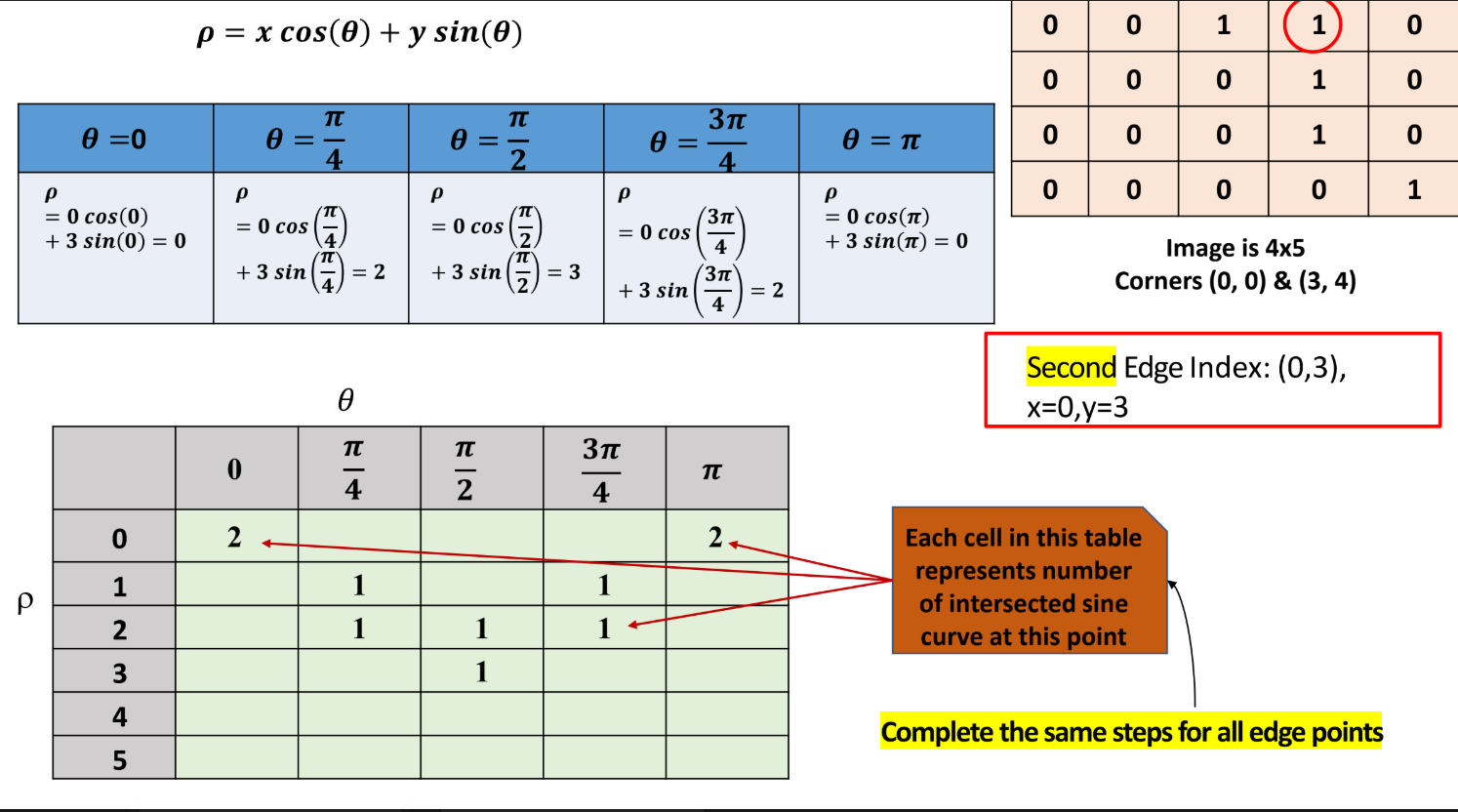
3. The Accumulation Process (The Math)

For every edge pixel $(x,y)$, the algorithm loops through every quantized $\theta$ value, calculates $\rho$ using the equation $\rho =x\cos (\theta )+y\sin (\theta )$ , rounds $\rho$ to the nearest integer , and increments that cell in the accumulator.

Processing the First Edge Point: $(0,2)$

• $\theta =0$: $\rho =0\cos (0)+2\sin (0)=0$. (Increment cell $\rho =0,\theta =0$)

• $\theta =\frac{\pi }{4}$: $\rho =0\cos (\frac{\pi }{4})+2\sin (\frac{\pi }{4})=2(0.707)=1.414\approx 1$. (Increment cell $\rho =1,\theta =\frac{\pi }{4}$)

• $\theta =\frac{\pi }{2}$: $\rho =0\cos (\frac{\pi }{2})+2\sin (\frac{\pi }{2})=2(1)=2$. (Increment cell $\rho =2,\theta =\frac{\pi }{2}$)

• $\theta =\frac{3\pi }{4}$: $\rho =0\cos (\frac{3\pi }{4})+2\sin (\frac{3\pi }{4})=2(0.707)=1.414\approx 1$. (Increment cell $\rho =1,\theta =\frac{3\pi }{4}$)

• $\theta =\pi$: $\rho =0\cos (\pi )+2\sin (\pi )=0$. (Increment cell $\rho =0,\theta =\pi$)

Processing the Second Edge Point: $(0,3)$

• $\theta =0$: $\rho =0\cos (0)+3\sin (0)=0$.

• $\theta =\frac{\pi }{4}$: $\rho =0\cos (\frac{\pi }{4})+3\sin (\frac{\pi }{4})=3(0.707)=2.121\approx 2$.

• $\theta =\frac{\pi }{2}$: $\rho =0\cos (\frac{\pi }{2})+3\sin (\frac{\pi }{2})=3(1)=3$.

• $\theta =\frac{3\pi }{4}$: $\rho =0\cos (\frac{3\pi }{4})+3\sin (\frac{3\pi }{4})=3(0.707)=2.121\approx 2$.

• $\theta =\pi$: $\rho =0\cos (\pi )+3\sin (\pi )=0$.

Note: As this process repeats for the remaining pixels $(1,3)$, $(2,3)$, and $(3,4)$, the accumulator grid fills up, representing the number of sinusoidal curves intersecting at those specific parameter bins.

4. Thresholding to Find Lines

Once the accumulator is fully populated, a threshold is applied to find the strongest lines. The slides specify a threshold of 3. Any value in the final matrix where the intersection count is $\ge 3$ is set to 1 (indicating a valid line), and everything else is set to 0.

(Note: The slides explicitly state that the final $6\times 5$ matrix shown on slide 17 is "not accurate for the given example" and is instead a conceptual placeholder to demonstrate how the final thresholding step converts a high-value accumulator into a binary output ).

Note: This same principle can be adapted for circle detection by expanding the parameter space to 3D to account for the circle equation $(x_i-a{)}^2+(y_i-b{)}^2=r^2$ where the parameters are $(a,b,r)$.

2. Region-Based Segmentation (Similarity)

When edges are too noisy or disconnected, finding boundaries fails. Region-based segmentation takes the opposite approach: it groups pixels together that share similar attributes (like intensity, color, or texture).

Simple Global Thresholding

This is the most basic form of segmentation. If you have light objects on a dark background, you separate them by choosing a threshold $T$.

• If $f(x,y)>T$, it becomes the object (e.g., 1 or white).

• If $f(x,y)\le T$, it becomes the background (e.g., 0 or black).

• Multilevel Thresholding uses multiple thresholds ($T_1,T_2$) to separate multiple distinct objects from the background.

Automatic Threshold Calculation: Instead of guessing $T$, an algorithm can compute it automatically using the image's histogram:

1. Compute the average gray level (${\mu }_1$) for pixels in the background and the average gray level (${\mu }_2$) for pixels in the object.

2. Set the threshold exactly in the middle: $T=\frac{{\mu }_1+{\mu }_2}{2}$.

3. Apply this threshold to create the binary image.

Region Growing

When simple thresholding fails (e.g., due to uneven lighting or severe noise), Region Growing is used.

1. Seed Selection: The algorithm starts with a set of specific starting pixels called "seed" points.

2. Aggregation: It looks at the neighboring pixels around the seed. If the absolute difference between the neighbor's gray level and the seed's gray level falls within a strict similarity threshold, that neighbor is "appended" to the growing region.

3. Iteration: This process spreads outward like a puddle until no more adjacent pixels meet the similarity criteria.