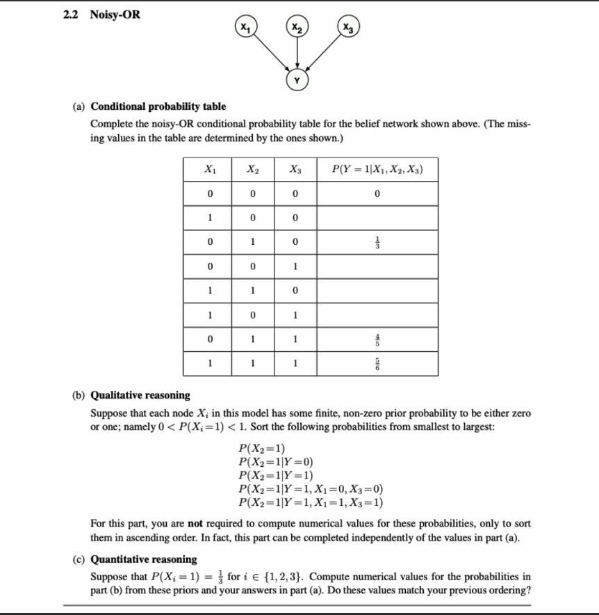
(a) Conditional Probability Table

In a Noisy-OR model, the probability that the effect $Y$ is absent ($Y=0$) is the product of the independent failure probabilities of each active cause $X_i$.

Let $q_i$ be the probability that $Y=0$ given that only $X_i=1$. The general Noisy-OR formula is:

First, we extract the failure probabilities $q_1,q_2,q_3$ from the given rows:

1. Find $q_2$:
   $P(Y=1\mid 0,1,0)=\frac{1}{3}⟹P(Y=0\mid 0,1,0)=\frac{2}{3}$. Therefore, $q_2=\frac{2}{3}$.
2. Find $q_3$:
   $P(Y=1\mid 0,1,1)=\frac{4}{5}⟹P(Y=0\mid 0,1,1)=\frac{1}{5}$.
   Using the Noisy-OR formula: $q_2\cdot q_3=\frac{1}{5}⟹\frac{2}{3}\cdot q_3=\frac{1}{5}⟹$ $q_3=\frac{3}{10}$.
3. Find $q_1$:
   $P(Y=1\mid 1,1,1)=\frac{5}{6}⟹P(Y=0\mid 1,1,1)=\frac{1}{6}$.
   Using the formula: $q_1\cdot q_2\cdot q_3=\frac{1}{6}⟹q_1\cdot \left(\frac{1}{5}\right)=\frac{1}{6}⟹$ $q_1=\frac{5}{6}$.

Now, we calculate the missing values in the table:

• Row 2 ($X_1=1,X_2=0,X_3=0$): $P(Y=1)=1-q_1=1-\frac{5}{6}=$ $\frac{1}{6}$
• Row 4 ($X_1=0,X_2=0,X_3=1$): $P(Y=1)=1-q_3=1-\frac{3}{10}=$ $\frac{7}{10}$
• Row 5 ($X_1=1,X_2=1,X_3=0$): $P(Y=1)=1-(q_1\cdot q_2)=1-(\frac{5}{6}\cdot \frac{2}{3})=1-\frac{5}{9}=$ $\frac{4}{9}$
• Row 6 ($X_1=1,X_2=0,X_3=1$): $P(Y=1)=1-(q_1\cdot q_3)=1-(\frac{5}{6}\cdot \frac{3}{10})=1-\frac{1}{4}=$ $\frac{3}{4}$

Completed Table:

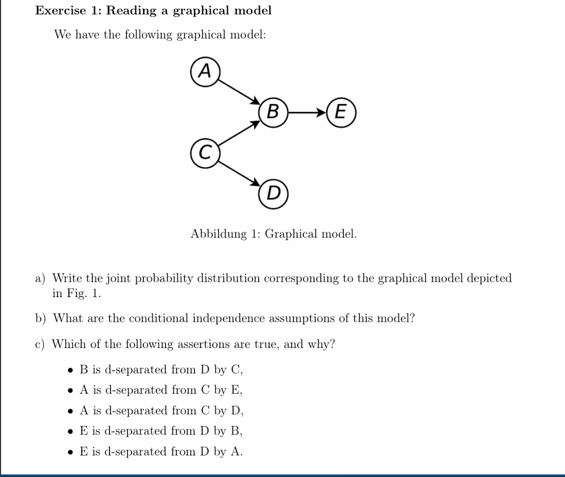
a) Joint Probability Distribution

The joint probability distribution for a Bayesian network is the product of the conditional probability distributions of each node given its parents.

Looking at the graph, we can identify the parents for each node:

• $A$: No parents

• $C$: No parents

• $B$: Parents are $A$ and $C$

• $D$: Parent is $C$

• $E$: Parent is $B$

Therefore, the joint probability distribution is:

b) Conditional Independence Assumptions

The fundamental assumption of a Bayesian network (the Local Markov Property) is that each node is conditionally independent of its non-descendants given its parents. Applying this rule to each node in the model gives us the following conditional independence assumptions:

• Node A: Has no parents. Its non-descendants are $C$ and $D$.

  • Assumption: $A\perp C,D$ (A is independent of C and D)

• Node C: Has no parents. Its non-descendant is $A$.

  • Assumption: $C\perp A$ (C is independent of A)

• Node B: Parents are $A,C$. Its non-descendant is $D$.

  • Assumption: $B\perp D\mid A,C$

• Node D: Parent is $C$. Its non-descendants are $A,B,E$.

  • Assumption: $D\perp A,B,E\mid C$

• Node E: Parent is $B$. Its non-descendants are $A,C,D$.

  • Assumption: $E\perp A,C,D\mid B$

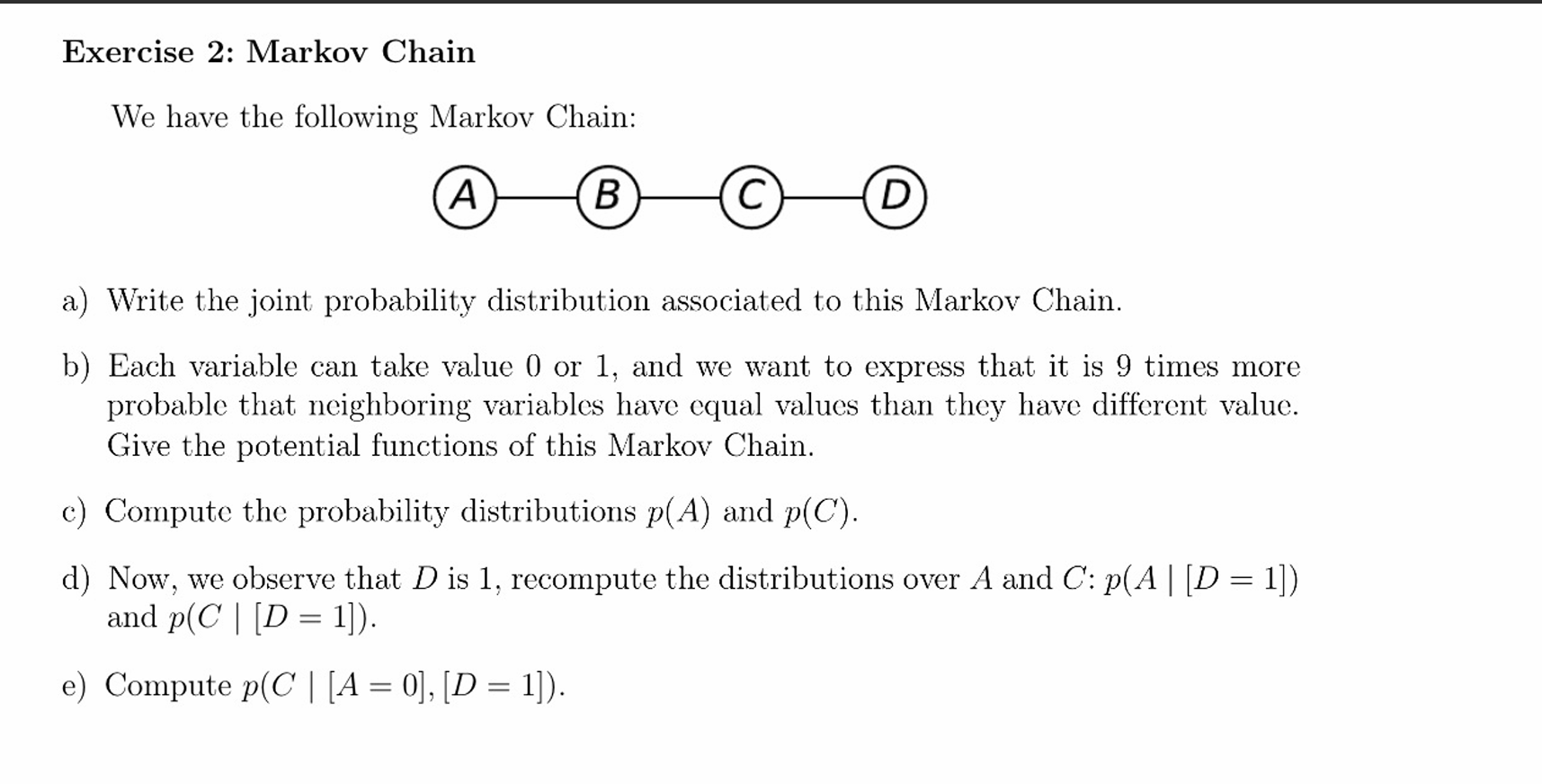
a) Joint Probability Distribution

In an undirected model, the joint probability distribution is factored into potential functions (often denoted as $\varphi$) over the maximal cliques (in this case, the pairs of connected nodes).

The joint probability distribution is:

Where $Z$ is the partition function (a normalization constant) that ensures all probabilities sum to 1:

b) Potential Functions

The problem states that each variable takes a value of 0 or 1, and it is 9 times more probable for neighboring variables to have equal values than different values.

Since the rule applies identically across the entire chain, we can use the same potential function for all pairs: $\varphi (A,B)=\varphi (B,C)=\varphi (C,D)$.

We can define the potential function $\varphi (X,Y)$ as:

• $\varphi (X,Y)=9$ if $X=Y$

• $\varphi (X,Y)=1$ if $X\ne Y$

Expressed as a table (or matrix) where the rows represent $X\in \{0,1\}$ and columns represent $Y\in \{0,1\}$: