Meaning of "pushing summations inward"

The concept of "pushing summations inward" is the mathematical heart of why Variable Elimination is so much more efficient than the brute-force approach. At its core, it is an algorithmic optimization built entirely on the distributive property of multiplication over addition—the same fundamental rule that states $xy+xz=x(y+z)$.

Instead of distributing multiplication over a massive set of additions (which creates a combinatorial explosion), Variable Elimination factors out the terms that don't depend on the variable you are currently summing over.

Here is exactly what that means, mapping the algebra directly to the numerical example from slides 3 through 9.

1. The Brute Force Approach: "Un-pushed" Summations

In the lecture's example of the network $A\to B\to C$, the goal is to calculate the marginal probability $P(C)$.

To do this using the full joint distribution (Method 2, Slides 6 & 7), you define the marginal probability as the sum over all possible states of $A$ and $B$:

If we expand $P(A,B,C)$ into its initial factors, the equation looks like this:

The Algorithmic Flaw: Because the summations are entirely on the outside, the algorithm is forced to compute the inner product $[{\varphi }_1(A)\cdot {\varphi }_2(A,B)\cdot {\varphi }_3(B,C)]$ for every single combination of $A$, $B$, and $C$ before doing any addition. This generates an 8-row table ($2^3=8$) with 16 total multiplications.

2. Pushing the Summations Inward

To optimize this, we look at the variables involved in each factor.

Notice the innermost sum over $A$ ($\sum _A$). We ask: Do all the factors in the product depend on $A$?

The factor ${\varphi }_3(B,C)$ does not contain the variable $A$. Because ${\varphi }_3(B,C)$ acts as a constant relative to $A$, we can factor it out and move it to the left of the $\sum _A$ operator.

We have successfully "pushed" the sum over $A$ inward:

3. Mapping to the Numerical Example (Method 1)

That newly restructured equation dictates the exact, step-by-step Variable Elimination algorithm shown in Slides 4 and 5. By isolating subproblems, we prevent the table size from exploding.

Step 1: The Inner Bracket (Eliminating A - Slide 4)

The innermost operation is now isolated: $[\sum _A{\varphi }_1(A)\cdot {\varphi }_2(A,B)]$.

1. Product: We multiply the factors that actually care about $A$: $\psi (A,B)={\varphi }_1(A)\cdot {\varphi }_2(A,B)$. This only requires calculating combinations of $A$ and $B$ (max size $2^2=4$).

2. Sum-out: We marginalize $A$ out of that product to create a new, intermediate factor: ${\tau }_1(B)=\sum _A\psi (A,B)$.

Step 2: The Outer Bracket (Eliminating B - Slide 5)

We substitute our new factor ${\tau }_1(B)$ back into the main equation. The equation is now simpler:

1. Product: We multiply the remaining factors that involve $B$: $\psi (B,C)={\tau }_1(B)\cdot {\varphi }_3(B,C)$. Again, this table only tracks $B$ and $C$ (max size $2^2=4$).

2. Sum-out: We marginalize $B$ out to get our final target: ${\tau }_2(C)=\sum _B\psi (B,C)$. This yields $P(C)=\{0.65,0.35\}$.

The Efficiency Payoff

By pushing the summations inward, we isolate the mathematical operations into decoupled blocks.

As shown in Slide 8, instead of generating a monolithic $2^3=8$ row table, we generated two smaller operations that each only required a maximum table size of $2^2=4$. If we had 50 variables in a chain, the brute-force equation would require calculating a $2^{50}$ row table before adding anything together. By pushing summations inward, Variable Elimination guarantees we only ever compute localized products between directly connected variables.

Why does the order in which we eliminate variables matter so much

The order in which you eliminate variables is the single most important factor in Variable Elimination because it directly dictates the computational cost (both time and memory) of the algorithm.

To put it simply: a good elimination order makes a problem trivially easy to solve, while a bad order can make the exact same problem mathematically impossible for a computer to process.

Here is a breakdown of why this happens:

1. It Dictates the Size of Intermediate Tables

Every time you eliminate a variable, you have to multiply all the factors that involve that variable together.

• If you eliminate a variable that is connected to only one or two other variables, you create a small intermediate table (e.g., a table with $2^2=4$ rows).

• If you eliminate a variable that is connected to many other variables—like a central "hub" in your network—you are forced to multiply all those related factors together at once. This creates a massive intermediate table.

2. The "Fill-in Edge" Effect and Induced Width

When you eliminate a variable from the graph, you conceptually "marry" all of its neighbors, creating what are called fill-in edges. All of those neighbors are merged into a single clique.

The complexity of the Variable Elimination algorithm is completely determined by the maximum factor size generated during the entire process. In graph theory, the size of the largest clique created during elimination is related to the graph's induced width. The time and memory required scale exponentially with this width.

3. Avoiding the Exponential Wall

Imagine a network shaped like a star, where one central node $A$ connects to 20 outer nodes.

• A Bad Order: If you choose to eliminate the central node $A$ first, you must multiply all 20 outer nodes together into one gigantic factor. You suddenly have to calculate and store a table with $2^{20}$ rows (over 1 million entries).

• A Good Order: If you eliminate the 20 outer nodes one by one first, you only ever deal with small, 2-variable factors (tables of 4 rows). The math is done in fractions of a second.

This is why, in the lecture's student performance example, eliminating the unobserved leaf node $S$ first was highly efficient—it didn't force any other variables to merge. Finding the absolute optimal elimination order is actually an NP-hard problem, but using heuristic strategies (like eliminating nodes with the fewest neighbors first) prevents the algorithm from crashing your computer's memory.

Purpose of Moralization

The primary purpose of moralization is to convert a directed Bayesian Network into an undirected graph so that the Variable Elimination (VE) algorithm can process it correctly.

Here is why this step is mathematically necessary:

• A Unified Framework: Variable Elimination is designed to treat both Bayesian Networks (directed) and Markov Networks (undirected) using the exact same algebraic framework, which relies on "factors".

• The Problem with Parents: In a Bayesian Network, a node's Conditional Probability Table (CPT), denoted as $P(X|P{a}_X)$, relies on the node itself ($X$) and all of its parents ($P{a}_X$).

• The Clique Requirement: In the language of undirected graphs, a factor can only exist if all the variables within its scope are directly connected to one another, forming a "clique".

How Moralization Solves This:

If two parent nodes share a child, they are part of the same CPT, but they might not be directly connected to each other in the original directed graph.

Moralization fixes this by "marrying the parents". You draw a new undirected edge between any parents that share a child, and then you drop the directional arrows from all other edges.

For example, in the lecture's student performance network, Intelligence ($I$) and Difficulty ($D$) both point to Grade ($G$), so they appear together in the factor $P(G|D,I)$. Moralization requires adding an edge between $I$ and $D$ to ensure that their dependency is captured correctly when they are merged into the Grade factor during calculation.

"Student Performance" example

1. Network Setup and Moralization (Slides 12–14)

The example uses a 5-node Bayesian Network representing a student's academic path. The variables are Difficulty ($D$), Intelligence ($I$), SAT/Score ($S$), Grade ($G$), and Letter ($L$). All variables are binary, meaning they can be either 0 (false/poor) or 1 (true/good).

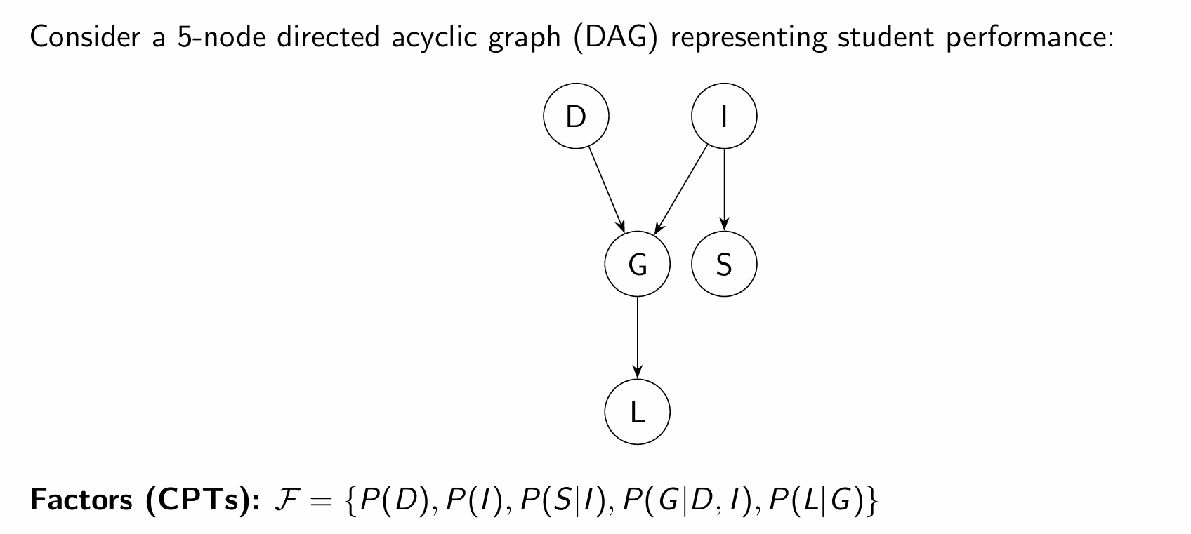
To prepare for Variable Elimination, the directed graph is "moralized" into an undirected graph. Because $D$ and $I$ share the child node $G$, they are "married" by adding an undirected edge between them. This ensures that the conditional probability table $P(G|D,I)$ forms a complete clique containing all three related variables.

2. The Query and Strategy (Slide 15)

The goal is to calculate the marginal probability of the student getting a good recommendation letter, or $P(L=1)$. To do this, we must sum out (marginalize) all other variables: $S$, $I$, $D$, and $G$.

The chosen elimination order is $S,I,D,G$. Applying the principle of pushing summations inward, the mathematical equation looks like this:

3. Step-by-Step Execution (Slides 16–19)

Step 1: Eliminating S (The Barren Node)

• Action: Isolate the factor involving $S$, which is ${\varphi }_S(S,I)$, and sum it out to create a new factor ${\tau }_1(I)$.

• Math: ${\tau }_1(I)=\sum _S{\varphi }_S(S,I)$.

  • For $I=0$: $P(S=0|I=0)+P(S=1|I=0)=0.8+0.2=1.0$.

  • For $I=1$: $P(S=0|I=1)+P(S=1|I=1)=0.1+0.9=1.0$.

• Insight: Because $S$ is a "leaf node" (it has no children) and is unobserved (we don't know the SAT score), summing it out results in a factor of 1s. This proves the "Barren Node Rule"—$S$ has no mathematical impact on the final calculation.

Step 2: Eliminating I

• Action: Multiply the factors involving $I$: ${\varphi }_I(I)$, ${\varphi }_G(G,D,I)$, and our new factor of 1s from the previous step, then sum out $I$. This creates a new 2-variable factor ${\tau }_2(G,D)$.

• Math: ${\tau }_2(G,D)=\sum _I{\varphi }_I(I)\cdot {\varphi }_G(G,D,I)$.

  • Calculating for $G=1,D=0$: We use the prior probabilities for $I$ ($P(I=1)=0.7$, meaning $P(I=0)=0.3$). ${\tau }_2(G^1,D^0)=P(I^0)P(G^1|D^0,I^0)+P(I^1)P(G^1|D^0,I^1)$. $=(0.3)(0.3)+(0.7)(0.9)=0.09+0.63=0.72$.

  • Calculating for $G=1,D=1$: ${\tau }_2(G^1,D^1)=P(I^0)P(G^1|D^1,I^0)+P(I^1)P(G^1|D^1,I^1)$. $=(0.3)(0.05)+(0.7)(0.5)=0.015+0.35=0.365$.

We only explicitly calculated the values for $G=1$ during the elimination of $I$ as a mathematical shortcut, not because $G=0$ doesn't exist.

Here is the full breakdown of why that shortcut works, and how it aligns with the lecture summary you provided.

1. The Shortcut: Why We Skipped $G=0$

When we eliminate $I$, the resulting factor ${\tau }_2(G,D)$ technically contains four values, covering every combination of $G$ and $D$:

• $G=1,D=1$

• $G=1,D=0$

• $G=0,D=1$

• $G=0,D=0$

However, the professor knew that the very next step was to eliminate $D$ to create ${\tau }_3(G)$. Because we have not introduced any strict evidence (like knowing for a fact the student failed), the factor ${\tau }_3(G)$ is mathematically equivalent to the actual marginal probability $P(G)$.

One of the foundational rules of probability is that all possible states of a single variable must sum to exactly 1. Therefore:

By calculating only the $G=1$ half of the ${\tau }_2(G,D)$ table, the professor had exactly enough information to find ${\tau }_3(G=1)$ (which was $0.507$). Instead of grinding through the math for $G=0$, they simply subtracted $0.507$ from $1$ to get $0.493$. It was a trick to cut the manual calculation time in half.

In short, your instinct was completely correct: a full algorithmic execution would calculate $G=0$ during the elimination of $I$. The professor just used human intuition to skip it.

Step 3: Eliminating D

• Action: Multiply the remaining factors involving $D$: ${\varphi }_D(D)$ and our new ${\tau }_2(G,D)$, then sum out $D$. This creates a 1-variable factor ${\tau }_3(G)$.

• Math: ${\tau }_3(G)=\sum _D{\varphi }_D(D)\cdot {\tau }_2(G,D)$.

  • Calculating for $G=1$: We use the prior probabilities for $D$ ($P(D=1)=0.6$, meaning $P(D=0)=0.4$). ${\tau }_3(G^1)=P(D^0){\tau }_2(G^1,D^0)+P(D^1){\tau }_2(G^1,D^1)$. $=(0.4)(0.72)+(0.6)(0.365)=0.288+0.219=0.507$.

  • Calculating for $G=0$: Because the total probabilities must sum to 1, ${\tau }_3(G^0)=1-0.507=0.493$.

To understand why the intermediate factor ${\tau }_3(G)$ is exactly equal to the real-world marginal probability $P(G)$, we have to look at what Variable Elimination is actually doing under the hood.

Variable Elimination is not an approximation; it is algebraically identical to calculating the full joint distribution and marginalizing variables out, just done in a smarter order.

Here is the step-by-step mathematical proof of why ${\tau }_3(G)=P(G)$, based on the network structure in the lecture.

The Mathematical Proof

If we want to find the true marginal probability $P(G)$ for the Grade node, we must sum over all of its ancestors (Intelligence and Difficulty). Because $D$ and $I$ are independent parent nodes, the true probability is defined as:

Now, let's look at how the Variable Elimination algorithm built ${\tau }_3(G)$ in the lecture example:

1. The creation of ${\tau }_2(G,D)$ When eliminating $I$, the algorithm multiplied the prior of $I$ with the Conditional Probability Table (CPT) for $G$, and summed out $I$:

2. The creation of ${\tau }_3(G)$ Next, when eliminating $D$, the algorithm took the prior of $D$, multiplied it by our new ${\tau }_2(G,D)$ factor, and summed out $D$:

3. Combining the equations

If we substitute the mathematical definition of ${\tau }_2(G,D)$ directly into the equation for ${\tau }_3(G)$, we get this:

Because of the distributive property, we can pull the summations to the outside and group the probabilities:

This final equation perfectly matches the definition of $P(G)$. By systematically pushing the summations inward, the algorithm naturally computed the exact marginal probability of the Grade node.

The "No Evidence" Condition

This equivalency only happened because no evidence was observed in any of the ancestor nodes ($D$, $I$, or $S$) prior to calculating $G$.

If we had observed evidence—for example, if we knew the student was highly intelligent ($I=1$)—the math would change:

• We would not sum over $I$. We would restrict the table to only the $I=1$ values.

• As a result, the final factor ${\tau }_3(G)$ would no longer represent the general probability $P(G)$.

• Instead, it would represent the joint probability with the evidence: $P(G,I=1)$.

Because there was no evidence acting as a constraint in the lecture's scenario, ${\tau }_3(G)$ maintained the properties of a pure probability distribution, allowing the professor to confidently use the shortcut ${\tau }_3(G^0)=1-0.507$.

Step 4: Final Elimination of G

• Action: We are left with our target factor ${\varphi }_L(L,G)$ and the intermediate factor ${\tau }_3(G)$. We sum out $G$ specifically for the condition $L=1$.

• Math: $P(L=1)=\sum _G{\tau }_3(G)\cdot P(L=1|G)$.

  • $P(L=1)={\tau }_3(G^0)P(L^1|G^0)+{\tau }_3(G^1)P(L^1|G^1)$.

  • $=(0.493)(0.1)+(0.507)(0.9)$.

  • $=0.0493+0.4563=0.5056$.

The Conclusion

The calculation reveals that there is approximately a 50.6% chance of the student receiving a good recommendation letter.

As slide 20 summarizes, this specific elimination order was highly efficient. By eliminating the cheap leaf node $S$ first, and isolating operations, the algorithm never had to build the full 32-row joint distribution table ($2^5=32$). The largest intermediate table it ever constructed had only 8 rows ($2^3=8$), which occurred during the elimination of $I$ when factors $G$, $D$, and $I$ were briefly evaluated together.