HMM Numerical Example

The Scenario Setup

Imagine a robot that is stationed inside a building without any windows. Its goal is to determine the hidden state of the world: Is it Raining ( $R$ ) outside?. Because the robot cannot observe the weather directly, the true weather state is considered a "hidden variable".

However, the robot can observe "evidence." In this case, the robot can see if people walking into the building are carrying Umbrellas ( $U$ ).

To solve this, the HMM uses two distinct probability models:

The Transition Model ( $P (R_{t} | R_{t - 1})$ ): How weather behaves over time.
- If it rained yesterday, there is a 70% chance it rains today: $P (R_{t} | R_{t - 1}) = 0.7$ .
- If it did not rain yesterday, there is a 30% chance it starts raining today: $P (R_{t} | \neg R_{t - 1}) = 0.3$ .
The Sensor/Observation Model ( $P (U_{t} | R_{t})$ ): How the weather influences people's behavior.
- If it is raining, there is a 90% chance people carry umbrellas: $P (U | R) = 0.9$ .
- If it is not raining, there is still a 20% chance people carry umbrellas (perhaps to block the sun): $P (U | \neg R) = 0.2$ .

The Initial Belief: The robot starts with a prior belief that there was a 50% chance of rain yesterday, meaning $P (R_{t - 1}) = 0.5$ . Today, the robot observes someone carrying an umbrella ( $U_{t} = true$ ).

Here is how the robot calculates the updated probability that it is currently raining, denoted mathematically as $P (R_{t} | U_{t})$ .

Step 1: Prediction (The Time Update)

Before the robot even looks at the umbrellas, it must forecast today's weather based purely on yesterday's belief and how weather naturally transitions. It does this using the Law of Total Probability to sum up all possible ways it could rain today.

P (R_{t}) = \sum_{r_{t - 1}} P (R_{t} | r_{t - 1}) P (R_{t - 1})

Expanded, this means the probability of rain today is the sum of two scenarios: (1) it rained yesterday and continued, OR (2) it didn't rain yesterday but started today.

P (R_{t}) = (P (R_{t} | R_{t - 1}) \times P (R_{t - 1})) + (P (R_{t} | \neg R_{t - 1}) \times P (\neg R_{t - 1}))

Plugging in the numbers from the models:

P (R_{t}) = (0.7 \times 0.5) + (0.3 \times 0.5)

P (R_{t}) = 0.35 + 0.15 = 0.5

So, based purely on time passing, the robot believes there is a 50% chance of rain today. This also inherently means there is a 50% chance of no rain today ( $P (\neg R_{t}) = 0.5$ ).

Step 2: The Update (Using the Observation)

Now, the robot looks at the door and observes an umbrella ( $U_{t}$ ). It uses Bayes' Rule to update its 50% belief by factoring in how likely it is to see an umbrella under different weather conditions.

The formula introduces an unnormalized constant, $α$ .

P (R_{t} | U_{t}) = α P (U_{t} | R_{t}) P (R_{t})

The robot calculates the "unnormalized" likelihoods for both possible realities (Rain vs. No Rain):

Reality 1: It is raining.

P (R_{t} | U_{t}) = α (0.9 \times 0.5) = 0.45 α

Reality 2: It is NOT raining.

P (\neg R_{t} | U_{t}) = α P (U_{t} | \neg R_{t}) P (\neg R_{t})

P (\neg R_{t} | U_{t}) = α (0.2 \times 0.5) = 0.1 α

Step 3: Normalization

In probability, the total chance of all possible states must equal exactly 1 (or 100%). Currently, our unnormalized values ( $0.45$ and $0.1$ ) do not sum to 1. The constant $α$ is used to force them to sum to 1.

We find $α$ by dividing 1 by the sum of our unnormalized values:

α = \frac{1}{0.45 + 0.1} = \frac{1}{0.55}

Finally, we apply this normalization factor to our "Rain" calculation to get the true percentage:

P (R_{t} | U_{t}) = \frac{0.45}{0.55} \approx 0.818

The Conclusion: Before seeing the umbrella, the robot thought there was a 50% chance of rain. After seeing the umbrella—because the sensor model tells the robot that umbrellas are a very strong indicator of rain—its confidence skyrocketed to approximately 81.8%.

Dynamic BN Example

Pasted image 20260416002553.png

The Scenario Setup

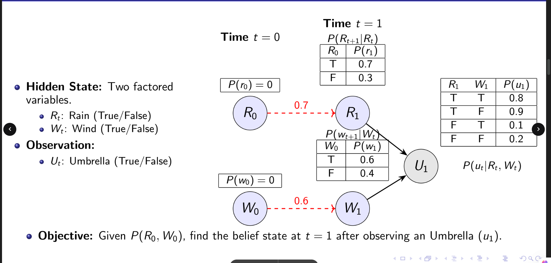
The DBN example builds on the HMM scenario but introduces a factored representation. Instead of a single hidden variable, the true state of the weather is split into two independent variables: Rain ( $R_{t}$ ) and Wind ( $W_{t}$ ).

The robot still observes Umbrellas ( $U_{t}$ ), but the likelihood of seeing an umbrella is now jointly influenced by both rain and wind.

The Initial Belief ( $t = 0$ ):

The robot starts with absolute certainty that it is neither raining nor windy.

$P (r_{0}) = 0$ .
$P (w_{0}) = 0$ .

The Transition Models: Rain and wind evolve over time completely independently of one another.

Rain: If it did not rain yesterday, there is a 30% chance it starts today ( $P (R_{t + 1} | \neg R_{t}) = 0.3$ ).
Wind: If it was not windy yesterday, there is a 40% chance it gets windy today ( $P (W_{t + 1} | \neg W_{t}) = 0.4$ ).

The Observation Model ( $P (U_{t} | R_{t}, W_{t})$ ): The chance of seeing an umbrella changes based on the combination of weather:

Rain + Wind: $0.8$ (Wind might break umbrellas, slightly lowering usage).
Rain + No Wind: $0.9$ .
No Rain + Wind: $0.1$ .
No Rain + No Wind: $0.2$ .

Step 1: Prediction ( $t = 0 \to t = 1$ )

Because the robot knew with 100% certainty that yesterday was clear and calm ( $P (\neg r_{0}, \neg w_{0}) = 1.0$ ), predicting today's weather prior to observing anything relies entirely on the transition probabilities from a "False" state.

First, calculate the individual probabilities for today:

$P (r_{1}) = 0.3$ .
$P (w_{1}) = 0.4$ .

Next, because the transitions are independent, you multiply them to find the "Joint Prior" representing the four possible realities for today's weather:

Rain & Wind ( $r_{1}, w_{1}$ ): $0.3 \times 0.4 = 0.12$ .
Rain & No Wind ( $r_{1}, \neg w_{1}$ ): $0.3 \times (1 - 0.4) = 0.18$ .
No Rain & Wind ( $\neg r_{1}, w_{1}$ ): $(1 - 0.3) \times 0.4 = 0.28$ .
No Rain & No Wind ( $\neg r_{1}, \neg w_{1}$ ): $0.7 \times 0.6 = 0.42$ .

Step 2: The Update (Using the Observation)

The robot now observes an Umbrella ( $u_{1}$ ). To update its beliefs, it uses Bayes' Rule to multiply the prior probability of each reality by the likelihood of seeing an umbrella in that specific reality.

This creates the unnormalized posterior ( $P^{'}$ ):

Reality 1 ( $r_{1}, w_{1}$ ): $0.8 \times 0.12 = 0.096$ .
Reality 2 ( $r_{1}, \neg w_{1}$ ): $0.9 \times 0.18 = 0.162$ .
Reality 3 ( $\neg r_{1}, w_{1}$ ): $0.1 \times 0.28 = 0.028$ .
Reality 4 ( $\neg r_{1}, \neg w_{1}$ ): $0.2 \times 0.42 = 0.084$ .

Step 3: Normalization & Marginalization

To convert these unnormalized values into true probabilities, they must be scaled so they sum to 1.

First, sum the unnormalized values:

0.096 + 0.162 + 0.028 + 0.084 = 0.37

Next, divide each unnormalized value by the sum ( $0.37$ ) to get the normalized posterior:

$P (r_{1}, w_{1} | u_{1}) \approx 0.259$ .
$P (r_{1}, \neg w_{1} | u_{1}) \approx 0.438$ .
$P (\neg r_{1}, w_{1} | u_{1}) \approx 0.076$ .
$P (\neg r_{1}, \neg w_{1} | u_{1}) \approx 0.227$ .

Finally, the robot wants to answer its core question: Is it raining? To find the overall probability of rain, it performs marginalization. It sums the probabilities of the two possible realities where it is raining, effectively factoring the wind variable out of the final equation:

P (r_{1} | u_{1}) = 0.259 + 0.438 = 0.697

The Conclusion

At time $t = 0$ , the robot was certain it was not raining (0%). After the natural passage of time and observing an umbrella, the robot's belief in rain shifted to 69.7%. A key takeaway from this DBN is that even though rain and wind naturally evolve completely independently of each other, the single observation of the umbrella immediately "couples" them together in the posterior calculation.

HMM Numerical Example

The Scenario Setup

Step 1: Prediction (The Time Update)

Step 2: The Update (Using the Observation)

Step 3: Normalization

Dynamic BN Example

The Scenario Setup

Step 1: Prediction (t=0→t=1)

Step 2: The Update (Using the Observation)

Step 3: Normalization & Marginalization

The Conclusion

Step 1: Prediction ( $t = 0 \to t = 1$ )