Sensor Uncertainty

These terms all describe critical flaws in how a robot perceives the physical world, leading to the uncertainty discussed in the localization lecture. Here is exactly how each phenomenon breaks down:

1. Reflective Environments

Many robots use ultrasonic sensors (sonar) or LIDAR to measure distance by emitting a sound or light wave and waiting for the echo to return. However, in a "reflective environment"—such as a room with glass, polished metal, or very smooth walls—the surfaces act like a mirror to the signal.

If the robot's sensor hits one of these smooth surfaces at an angle (rather than perfectly straight on), the signal deflects away into the room instead of bouncing back to the receiver. Because the sensor never hears the echo, it falsely records that the path is completely clear, potentially causing the robot to drive straight into a wall.

هنا السيجنال مش بترجع للسينسور اساسا, فا مش بيلقط الجسم من الأساس, فا ممكن يخبط في حيطة او اي حاجة تانية لانه ببساطة مشافهاش

2. Multipath Interference

This is a closely related physics problem where the emitted signal does return to the sensor, but it takes a deceptive path.

Instead of hitting an obstacle and bouncing directly back to the robot, the wave bounces off the target, hits a side wall, and then returns to the receiver.

Robots calculate distance using the "Time of Flight" principle (calculating distance based on how many milliseconds the echo took to return). Because the multipath signal took a longer, zig-zagging route, the time of flight is artificially inflated. The robot processes this delayed signal and mathematically concludes that the obstacle is much further away than it actually is, creating a "ghost" reading in its map.

بالبلدي
(لما السينسور يبعت سيجنال عشان يلقط اللي قدامه, بدل ما السيجنال تتعكس من الجسم علطول, تتعكس علي اكتر من سطح تاني قبل ما يرجع للسينسور, فا السيجنال بتمشي اكتر من طريق على ما ترجع للسينسور, hence the name "Multipath"), مما بيخلي الروبوت يدرك المسافات بشكل خاطئ لانه بيعتمد علي المدة الي بتاخدها السيجنال عشان ترجع للسينسور, في تحديد المسافة بينه و بين الجسم.

3. Sensor Aliasing (Perceptual Aliasing)

Sensor aliasing occurs when completely different physical locations in the real world produce the exact same sensor readings.

Imagine a robot in a long, uniform office hallway. If it takes a reading, its distance sensors might simply report: "Solid wall 1 meter to the left, solid wall 1 meter to the right, open space ahead."

The problem is that this specific array of data will look identical whether the robot is exactly 2 meters down the hallway, 10 meters down the hallway, or 20 meters down the hallway. The sensor data is not unique. A single reading "aliases" (maps to) multiple valid coordinates on the map. Because of sensor aliasing, a robot can almost never figure out where it is from a single snapshot; it must combine multiple readings over time as it moves to filter out the duplicate possibilities.

بالبلدي,
القراية الواحدة في نقطة زمنية محددة مش كافية تقول للروبوت هو واقف فين بالضبط, زي المثال الي فوق, لو واقف في طرقة طويلة او في متاهة, ممكن اكتر من مكان يدوا نفس القراية بالضبط, مما يصعب علي الروبوت هو واقف في اني حتة في الطرقة بالضبط, او في اني حتة في المتاهة, لو مبصش علي بقية القرايات السابقة و اعتمد علي اللحظية بس

Numerical Examples

Colored Doors

Here is the new environment: Door 1 (Green), Door 2 (Red), Door 3 (Red), Door 4 (Green), Door 5 (Green).

The sensor flaw remains the same:

• Likelihood of seeing "Red" at a Red door = $0.6$
• Likelihood of seeing "Red" at a Green door = $0.2$

Let's assume the robot drops in, powers on, and immediately senses "Red".

Step 1: Initial Belief (The Prior)

With 5 doors and zero initial knowledge, the probability is distributed equally ($1/5$).

• Belief Map: [0.20, 0.20, 0.20, 0.20, 0.20]

Step 2: The Sense Step (Likelihood)

The robot senses "Red". It maps the sensor likelihood against the true color of each door in the array:

• Door 1 (G): $0.2$
• Door 2 (R): $0.6$
• Door 3 (R): $0.6$
• Door 4 (G): $0.2$
• Door 5 (G): $0.2$

Step 3: The Update Step ($Prior\times Likelihood$)

We multiply the initial belief by the likelihood for each respective door.

• Door 1: $0.20\times 0.2=0.04$
• Door 2: $0.20\times 0.6=0.12$
• Door 3: $0.20\times 0.6=0.12$
• Door 4: $0.20\times 0.2=0.04$
• Door 5: $0.20\times 0.2=0.04$

Step 4: Normalization

Right now, the total sum of these probabilities is $0.36$ ($0.04+0.12+0.12+0.04+0.04$). To make this a valid probability distribution that equals $1.0$ ($100\mathrm{\%}$), we divide each raw number by $0.36$.

• Door 1: $0.04/0.36=1/9\approx 11.11\mathrm{\%}$
• Door 2: $0.12/0.36=3/9\approx 33.33\mathrm{\%}$
• Door 3: $0.12/0.36=3/9\approx 33.33\mathrm{\%}$
• Door 4: $0.04/0.36=1/9\approx 11.11\mathrm{\%}$
• Door 5: $0.04/0.36=1/9\approx 11.11\mathrm{\%}$

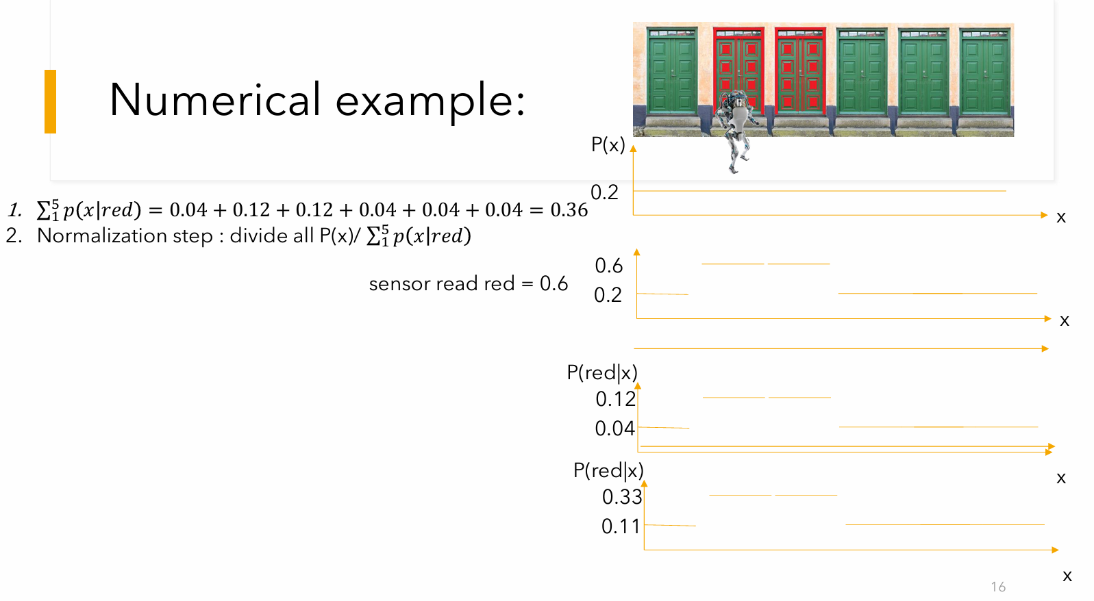
At this point, the robot is equally torn between Door 2 and Door 3. It knows it is highly likely to be at a Red door, but because there are two of them adjacent to each other, a single sensor reading suffers from sensor aliasing. It cannot mathematically distinguish between Door 2 and Door 3 yet.

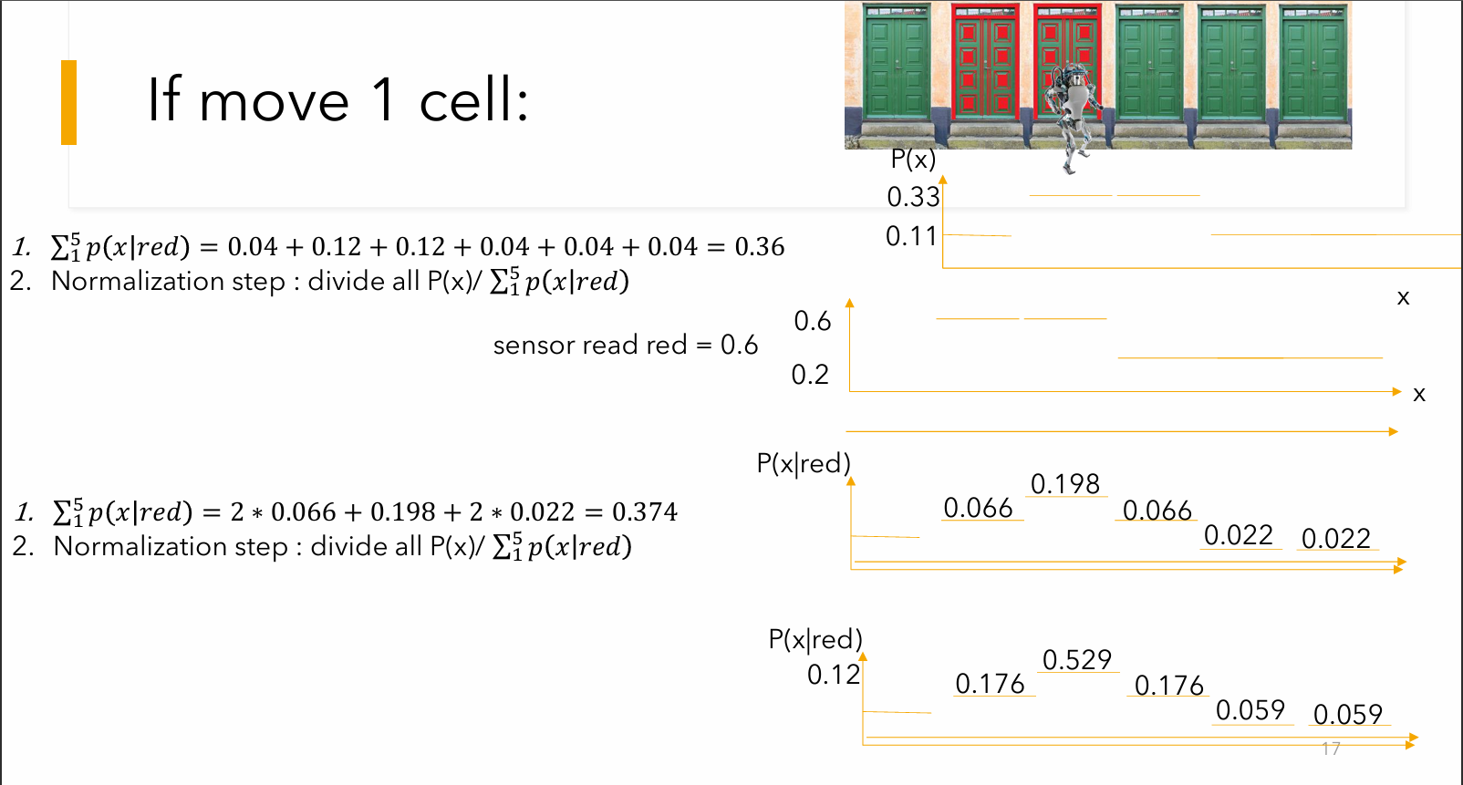
Step 5: The Move Step (Prediction)

To break the tie, the robot rolls forward by one door. Assuming its odometry is perfect and the wheels don't slip, the probabilities perfectly shift one slot to the right.

• New Belief Map: [11.11%, 11.11%, 33.33%, 33.33%, 11.11%] (assuming looped)

The Tie-Breaker (Next Loop)

Now, imagine the robot takes a second reading and senses "Red" again.

It will repeat the math, but this time, the updated belief map is the new prior. When it multiplies the likelihoods, Door 3 (which is Red and currently holds $33.33\mathrm{\%}$ probability) will receive a massive mathematical boost ($0.3333\times 0.6$). Door 2 (which is Red, but currently only holds $11.11\mathrm{\%}$ probability because the robot moved away from the first spot) will get a much smaller boost ($0.1111\times 0.6$).

After normalizing this second round, the probability will spike drastically on Door 3, allowing the robot to confidently "localize" itself and break the aliasing illusion!

Slide 18 from the lecture contains several massive arithmetic errors: the professor's multiplication terms do not match the doors, the sum is calculated incorrectly (writing 0.426 instead of 0.33 or 0.506), and the final probabilities on the slide only add up to roughly 77.5% instead of 100%.

The Initial Setup

• Cell 0 (Green): 1/9 (11.1%)

• Cell 1 (Red): 3/9 (33.3%)

• Cell 2 (Red): 3/9 (33.3%)

• Cell 3 (Green): 1/9 (11.1%)

• Cell 4 (Green): 1/9 (11.1%)

Step 1: The Move Step (Prediction)

You asked what happens if the robot moves from Cell 1 to Cell 3. This is a movement of 2 steps to the right. (0 index)

Assuming perfect odometry (the wheels don't slip), we simply take the entire probability distribution and shift it 2 slots to the right. In a standard continuous loop, the probabilities falling off the right side wrap around to the left:

• Cell 0 (Green) gets Cell 3's old probability: 1/9 (11.1%)

• Cell 1 (Red) gets Cell 4's old probability: 1/9 (11.1%)

• Cell 2 (Red) gets Cell 0's old probability: 1/9 (11.1%)

• Cell 3 (Green) gets Cell 1's old probability: 3/9 (33.3%)

• Cell 4 (Green) gets Cell 2's old probability: 3/9 (33.3%)

New Belief Map after moving: [11.1%, 11.1%, 11.1%, 33.3%, 33.3%]

Step 2: The Sense Step (Correction)

To follow the exact scenario on Slide 18, we now assume the robot takes a reading and senses "Green".

Based on the lecture's flawed sensor model, the likelihoods are:

• Sensing Green at a Green Door = 0.6

• Sensing Green at a Red Door = 0.2

We multiply the new shifted belief by the likelihood of sensing green for each specific door:

• Cell 0 (Green): $(1/9)\times 0.6=0.0667$

• Cell 1 (Red): $(1/9)\times 0.2=0.0222$

• Cell 2 (Red): $(1/9)\times 0.2=0.0222$

• Cell 3 (Green): $(3/9)\times 0.6=0.2000$

• Cell 4 (Green): $(3/9)\times 0.6=0.2000$

(Note: If you look closely at these numbers, you will see why the lecture slide is broken. Dr. Shiple's slide lists three 0.022s and only one 0.198. He lost track of his own doors while writing the slide!)

Step 3: Normalization

Right now, our raw numbers add up to 0.5111 ($0.0667+0.0222+0.0222+0.2000+0.2000$).

Because a probability distribution must always equal exactly 100%, we divide each individual number by the total sum (0.5111) to get the final, mathematically correct answer:

• Cell 0 (Green): $0.0667/0.5111=$ 13.0%

• Cell 1 (Red): $0.0222/0.5111=$ 4.3%

• Cell 2 (Red): $0.0222/0.5111=$ 4.3%

• Cell 3 (Green): $0.2000/0.5111=$ 39.2%

• Cell 4 (Green): $0.2000/0.5111=$ 39.2%

The robot is now heavily torn between Cell 3 and Cell 4, which makes perfect logical sense: it shifted its high probability mass over to those cells, and because both of those cells are Green doors, sensing "Green" heavily reinforced that belief!

2D Grid

The 2D grid example in the slides applies the exact same Markov Localization logic as the colored doors, but expands it from a 1D line into a two-dimensional space.

Here is a detailed breakdown of how this example works across the slides:

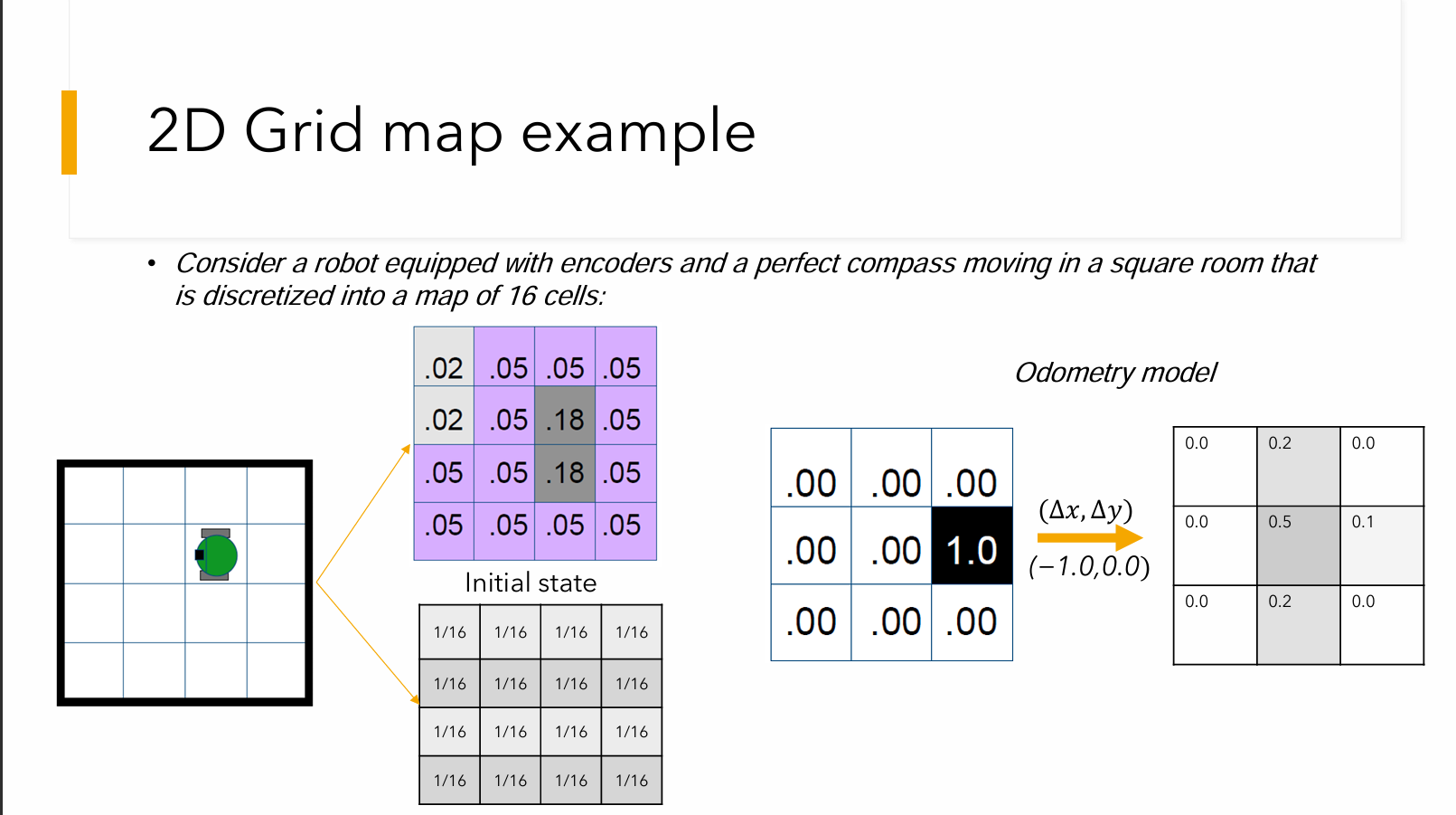
1. The Setup & Initial State

The scenario features a robot equipped with encoders (for tracking movement) and a perfect compass, navigating a square room that is discretized into a map of exactly 16 cells.

Because the robot starts with zero knowledge of its location, the "Initial state" is a uniform distribution. The total probability of $1.0$ (or $100\mathrm{\%}$) is divided equally among the 16 cells, meaning every single cell starts with a $1/16$ probability of containing the robot .

2. The Move Step (Prediction & Odometry Error)

When the robot attempts to move—for example, shifting one cell left, represented as $(\mathrm{\Delta }x,\mathrm{\Delta }y)=(-1.0,0.0)$ —the probability mass does not just cleanly shift one cell over.

Because of effector noise (like wheel slip), the slide introduces a 3x3 "Odometry model" matrix. This matrix dictates how the probability spreads out or "smears" when the robot moves. For example, the matrix shows:

• $0.5$: A 50% chance the robot lands exactly in the intended target cell.
• $0.2$: A 20% chance it drifts up, and a 20% chance it drifts down.
• $0.1$: A 10% chance it overshoots its movement.

Instead of the robot knowing it definitely moved one cell left, this Odometry model diffuses its belief across a small cluster of cells.

3. The Sense Step (Correction)

The robot then takes a reading with its external sensors. The slides provide a 4x4 likelihood matrix (the table containing values like $0.02$, $0.05$, and $0.18$). This grid represents the mathematical likelihood of receiving that exact sensor reading for every specific cell in the room. Notice how some cells have a higher likelihood ($0.18$), indicating the sensor reading strongly matches the physical features of those specific map coordinates.

4. The Correlation Step (Update)

Just like multiplying the prior belief by the likelihood in the door example, the algorithm now mathematically overlays the smeared prediction matrix (from the Move step) with the likelihood map (from the Sense step).

The slides walk through calculating this correlation, resulting in a new 4x4 matrix of raw probabilities where most of the numbers are $0.0$, but a few cells hold values like $0.09$, $0.036$, and $0.01$ .

5. Normalization

Because these raw correlation numbers do not add up to $1.0$, they must be normalized. The slide shows the sum of these probabilities is calculated: $\sum _1^{5}p(x|red)=0.01+0.09+0.36+0.005=0.141$ (Note: the slide contains a typo in the equation text, writing $0.36$ instead of $0.036$, but the sum $0.141$ is based on the grid values).

As noted in the summary slide, the final Normalization step requires dividing the belief state by this total sum: $P(x)/{\mathrm{\Sigma }}_1^{5}p(x|red)$. By repeating this cycle, the robot filters out its movement drift and zeros in on its true coordinates on the 2D map.